


Los modelos matemáticos de muchos sistemas geofísicos requieren el procesamiento de sistemas algebraicos de gran escala. Las herramientas computacionales más avanzadas están masivamente paralelizadas. El software más efectivo para resolver ecuaciones diferenciales parciales en paralelo intenta alcanzar el paradigma de los métodos de descomposición de dominio, que hasta ahora se había mantenido como un anhelo no alcanzado. Sin embargo, un grupo de cuatro algoritmos –los algoritmos DVS- que lo alcanzan y que tiene aplicabilidad muy general se ha desarrollado recientemente. Este artículo está dedicado a presentarlos y a ilustrar su aplicación a problemas que se presentan frecuentemente en la investigación y el estudio de la Geofísica.
Mathematical models of many geophysical systems are based on the computational processing of large-scale algebraic systems. The most advanced computational tools are based on massively parallel processors. The most effective software for solving partial differential equations in parallel intends to achieve the DDM-paradigm. A set of four algorithms, the DVS-algorithms, which achieve it, and of very general applicability, has recently been developed and here they are explained. Also, their application to problems that frequently occur in Geophysics is illustrated.
Mathematical models of many systems of interest, including very important continuous systems of Earth Sciences and Engineering, lead to a great variety of partial differential equations (PDEs) whose solution methods are based on the computational processing of large-scale algebraic systems. Furthermore, the incredible expansion experienced by the existing computational hardware and software has made amenable to effective treatment problems of an ever increasing diversity and complexity, posed by scientific and engineering applications [PITAC, 2006].
Parallel computing is outstanding among the new computational tools and, in order to effectively use the most advanced computers available today, massively parallel software is required. Domain decomposition methods (DDMs) have been developed precisely for effectively treating PDEs in parallel [DDM Organization, 2012]. Ideally, the main objective of domain decomposition research is to produce algorithms capable of ‘obtaining the global solution by exclusively solving local problems’, but up-to-now this has only been an aspiration; that is, a strong desire for achieving such a property and so we call it ‘the DDM-paradigm’. In recent times, numerically competitive DDM-algorithms are non-overlapping, preconditioned and necessarily incorporate constraints [Dohrmann, 2003; Farhat et al., 1991; Farhat et al., 2000; Farhat et al., 2001; Mandel, 1993; Mandel et al., 1996; Mandel and Tezaur, 1996; Mandel et al., 2001; Mandel et al., 2003; Mandel et al., 2005; J. Li et al., 2005; Toselli et al., 2005], which pose an additional challenge for achieving the DDM-paradigm.
Recently a group of four algorithms, referred to as the ‘DVS-algorithms’, which fulfill the DDM-paradigm, was developed [Herrera et al., 2012; L.M. de la Cruz et al., 2012; Herrera and L.M. de la Cruz et al., 2012; Herrera and Carrillo-Ledesma et al., 2012]. To derive them a new discretization method, which uses a non-overlapping system of nodes (the derived-nodes), was introduced. This discretization procedure can be applied to any boundary-value problem, or system of such equations. In turn, the resulting system of discrete equations can be treated using any available DDM-algorithm. In particular, two of the four DVS-algorithms mentioned above were obtained by application of the well-known and very effective algorithms BDDC and FETI-DP [Dohrmann, 2003; Farhat et al., 1991; Farhat et al., 2000; Farhat et al., 2001; Mandel et al., 1993; Mandel et al., 1996; Mandel and Tezaur, 1996; Mandel et al., 2001; Mandel et al., 2003; Mandel et al., 2005; J. Li et al., 2005; Toselli et al., 2005]; these will be referred to as the DVS-BDDC and DVS-FETI-DP algorithms. The other two, which will be referred to as the DVS-PRIMAL and DVS-DUAL algorithms, were obtained by application of two new algorithms that had not been previously reported in the literature [Herrera et al., 2011; Herrera et al., 2010; Herrera et al., 2009; Herrera et al., 2009; Herrera, 2008; Herrera, 2007]. As said before, the four DVS-algorithms constitute a group of preconditioned and constrained algorithms that, for the first time, fulfill the DDM-paradigm [Herrera et al., 2013; L.M. de la Cruz et al., 2012].
Both, BDDC and FETI-DP, are very well-known [Dohrmann, 2003; Farhat et al., 1991; Farhat et al., 2000; Farhat et al., 2001; Mandel et al., 1993; Mandel et al., 1996; Mandel and Tezaur, 1996; Mandel et al., 2001]; and both are highly efficient. Recently, it was established that these two methods are closely related and its numerical performance is quite similar [Mandel et al., 2003; Mandel et al., 2005]. On the other hand, through numerical experiments, we have established that the numerical performances of each one of the members of DVS-algorithms group (DVS-BDDC, DVS-FETI-DP, DVS-PRIMAL and DVS-DUAL) are very similar too. Furthermore, we have carried out comparisons of the performances of the standard versions of BDDC and FETI-DP with DVS-BDDC and DVS-FETI-DP, and in all such numerical experiments the DVS algorithms have performed significantly better.
Each DVS-algorithm possesses the following conspicuous features:
- •
It fulfills the DDM-paradigm;
- •
It is applicable to symmetric, non-symmetric and indefinite matrices (i.e., neither positive, nor negative definite); and
- •
It is preconditioned and constrained, and has update numerical efficiency.
Furthermore, the uniformity of the algebraic structure of the matrix-formulas that define each one of them is remarkable.
This article is organized as follows. In Section 2 the basic definitions for the DVS framework are given; here we define the set of ‘derived-nodes’, internal, interface, primal and dual nodes, the ‘derived-vector-space’, among others. Section 3 is devoted to define the new set of vector spaces that conforms the DVS framework; the Euclidean inner product, is also defined here. In Section 4 the ‘transformed-problem’ on the derived-nodes is explained in detail, and this is our starting point to define the DVS algorithms. Section 5 presents a summary of the four DVS-algorithms: DVS-BDDC, DVS-FETI-DP, DVS-PRIMAL and DVS-DUAL. In Section 6 we give the numerical procedures we use to fulfilling the DDM-paradigm, and we explain in detail the implementation issues. Finally, in Section 7 we show some numerical results obtained after the application of the DVS-algorithms in the solution of several boundary values problems of interest in Geophysics. We studied examples for a single-equation, for the cases of symmetric, non-symmetric and indefinite problems. We also present results for an elasticity problem, where a system of PDE equations is solved.
2DVS Framework: A SummaryThe ‘derived-vector-space framework (DVS-framework)’ is applied to the discrete system of equations that is obtained after the partial differential equation, or system of such equations, has been discretized. The procedure is independent of the method of discretization that is used. Thus, the DVS-framework’s starting point is a system of linear algebraic equations that is referred to as the ‘original problem’:

However, in the DVS setting one does not work with the set of nodes originally used for discretizing the problem the original-nodes’ (Figure 1). Instead, one uses an auxiliary set of nodes: the ‘derived-nodes’. Each one of such nodes has the property that it belongs to one and only one subdomain of the coarse mesh.

Indeed, generally after a coarse-mesh has been introduced, some original-nodes belong to more than one subdomain of the coarse-mesh (Figure 2), which is inconvenient for achieving the DDM-paradigm. Therefore, in the DVS-framework, each original-node that belongs to more than one subdomain is divided into as many new nodes – the derived-nodes (Figure 3) - as subdomains it belongs to. Then, the derived-nodes so obtained are distributed into the coarse-mesh subdomains so that each derived-node is assigned to one and only one subdomain of the coarse-mesh (Figure 4). Once this has been done, a convenient notation is to label each derived-node by a pair of natural numbers: the first one indicating the original-node from which it derives and the second one, the subdomain to which it is assigned.


The real-valued functions defined in the set of derived-nodes constitute a vector-space: the ‘derived-vector-space’, W. This space becomes a finite-dimensional Hilbert-space when it is supplied with the inner-product that is usually introduced when dealing with real-valued functions defined in a set of nodes; this is referred to as the Euclidean inner-product.
Afterwards, a new problem (referred to as the ‘transformed problem’) is defined in the derived-vector-space, which is equivalent to the original system of discrete equations. Thereafter, all the numerical and computational work is carried out in the DVS-space.
Before leaving this Section, we dwell a little further on the meaning of a coarse-mesh. By it, we mean a partition of Ω into a set of non-overlapping subdomains {Ω1,...,ΩE}, such that for each α=1, ..., E, Ωα′, is open and:
Where Ω¯α stands for the closure of Ωα. The set of ‘subdomain-indices’ will be

Nˆα, α=1,..., E, will be used for the subset of original-nodes that correspond to nodes pertaining to Ω¯α. As usual, nodes will be classified into ‘internal’ and ‘interface-nodes’: a node is internal if it belongs to only one partition-subdomain closure and it is an interface-node, when it belongs to more than one. For the application of dualprimal methods, interface-nodes are classified into ‘primal’ and ‘dual’ nodes. We define:
NˆI⊂Nˆ as the set of internal-nodes;
NˆΓ⊂Nˆ as the set of interface-nodes;
Nˆπ⊂NˆΓ⊂Nˆ as the set of primal-nodes1; and
NˆΔ⊂Nˆ as the set of dual-nodes.
The set of primal-nodes is required to be a subset of NˆΓ and, in principle, could be otherwise chosen arbitrarily. However, the algorithms considered by domain decomposition methods are iterative-algorithms and their rate of convergence depends crucially on the selection of the set Nˆπ. Thus, criteria for selecting Nˆπ have been studied extensively (see [Toselli et al., 2005], for detailed discussions of this topic). Each one of the following two families of node-subsets is disjoint :NˆI,NˆΓ and NˆI,Nˆπ,NˆΔ. Furthermore, these node subsets fulfill the relations:

Throughout our developments the original matrixA⌢__ is assumed to be non-singular (i.e., it defines a bijection of Wˆ into itself). The following assumption (‘axiom’) is also adopted in throughout the DVS-framework: “When the indices p∈Nˆα and q∈Nˆβ are internal original-nodes, while α ≠ β, then p∈Nˆα and q∈Nˆβ are unconnected”. We recall that unconnected means:
3The Derived-Vector Space (DVS)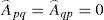
In order to have at hand a sufficiently general framework, we consider functions defined on the set X of derived-nodes whose value at each derived-node is a dD-Vector. The numerical applications that will be discussed in this paper correspond to two possible choices of d: when the application refers to a single partial differential equation (PDE), d=1, and for the problems of elasticity that will be considered, which are governed by a three-equations system, d=3.
Independently of the chosen value for d, the set of such functions constitute a vector space, W, referred to as the ‘derived-vector space’. When u_;∈W, we write u(p, α) for the value of u_; at the derived-node (p, α). We observe that, in general, u(p, α) itself is a d-Vector and we adopt the notation u(p, α, i), i=1, ..., d. For the i-th component of u(p, α). When d=1 the index i is irrelevant and, in such a case, will deleted throughout.
For every pair of functions, u_;∈W and w_;∈W, the ‘Euclidean inner product’ is defined to be
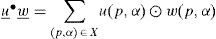
Here, u(p,α)⊙w(p,α) stands for the inner-product of the dD-Vectors involved; thus,
A fundamental property of the derived-vector space W, is that it constitutes a finite dimensional Hilbert-space with respect to the Euclidean innerproduct.
Let W′⊂W be a linear subspace and assume M⊂X is a subset of derived-nodes. Then, the notation W’(M) will be used to represent the vector subspace of W’, whose elements vanish at every derived-node that does not belong to M. Furthermore, corresponding to each local subset of derived-nodes, Xα, there is a ‘local subspace of derived-vectors’, Wα, which is defined by

Clearly, when u_;∈Wα⊂W, u_;(p,β)=0 whenever β ≠ α. We observe that
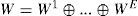
A derived-vector u_;∈W is said to be continuous when u_;(p,α) is independent of α. The set of continuous vectors constitute the linear subspace, W12.
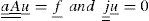
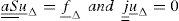
The orthogonal complement (with respect to the Euclidean inner-product) of W12⊂W is W11⊂W. Then W=W11⊕W12. Two projection-matrices a__:W→W and j__:W→W are here introduced; they are the projection-operators, with respect to the Euclidean inner-product on W12 and W11, respectively. When u_;∈W, one has
the vectors j__u_; and a__u_; are said to be the ‘jump’ and the ‘average’ of u_;, respectively. Therefore, W11 is the ‘zero-average’ subspace, while W12 is the ‘zero-jump’ subspace.
Original-nodes are classified into ‘internal’ and ‘interface-nodes’: a node is internal if it belongs to only one subdomain-closure of the coarse-mesh, and it is an interface-node when it belongs to more than one of such closure-subdomains. Some subspaces, significant for our developments, are listed next:
At present, numerically competitive algorithms need to incorporate restrictions and to this end, in the DVS-framework, a ‘restricted subspace’ Wr⊂W is selected. In the developments that follow, it is assumed that:
The matrix a__r will be the projection-operator on Wr. We observe that when u_;∈(WI+WΔ), one has a__ru_;=u_;. We also notice that
4The Transformed Problem
The transformed-problem consists in finding u_;∈W such that
Where:

and
together with
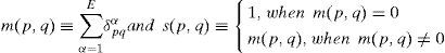
The function m (p, q) is said to be the ‘multiplicity’ of the pair (p, q). The ‘derived-nodes’ are created after a coarse-mesh has been introduced, by dividing the original-nodes as explained in the Overview (Section 2), and then with each ‘derived-node’ we associate a unique pair of numbers (p, α) such that α∈Eˆ and p∈Nˆα. In what follows, we identify derived-nodes with such pairs.
Then, in order to incorporate the constraints, we define

then, the matrix A__:Wr→Wr defined by

has the property that

Hence, Eq. (4.1) is replaced by
For matrices and vectors the following notation is adopted:
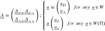
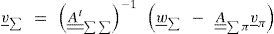
where the matrices
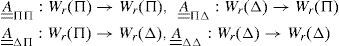
furthermore,
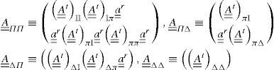
The matrix A__:W→W will be referred to as the ‘transformed-matrix’. We observe that A__=A__t when π = Ø.
In turn, the transformed problem of (4.8) can be reduced, see [Herrera et al., 2010; Herrera et al., 2009; Herrera, 2008; Herrera, 2007; Farhat et al., 2000] for details, into the following problem, which is expressed in terms of the values of the solution at dual-nodes, exclusively: “Find u_;Δ∈W (∆) that satisfies
Here, f_;Δ∈a__W(Δ) and the ‘Schur-complement matrix with constraints’ are defined by
and
respectively.
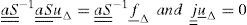
5The DVS-AlgorithmsGenerally two kinds of approaches are distinguished: primal –these are direct approaches, which do not resort to Lagrange multipliers- and dual –indirect approaches that use Lagrange multipliers-. However, when DDMs are formulated using a setting as general as that supplied by the DVS-framework, such a distinction is irrelevant. The feature that is conspicuous for different options is the information that the algorithm seeks. Indeed, four algorithms will be obtained by seeking successively for the vectors: u_;Δ,S__−1j__S__u_;Δ, j__S__u_;Δ, and S__u_;Δ. However, in the presentation that follows we stick to the ‘primal vs. dual-algorithms’ classification.
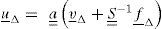
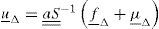
5.1Primal FormulationsThe DVS Version of BDDCThis is a primal algorithm which seeks directly for u_;Δ. Pre-multiplying Eq. (4.12) by a__S__−1, one gets:
In [Farhat et al., 2000], it was shown that Eq. (5.1) is equivalent to Eq. (4.12). This equation is the DVS-version of BDDC.
The DVS-Primal AlgorithmFor this algorithm, the sought-information is:
Applying to a__S__Eq. (5.2) it is seen that a__S__v_;Δ=0. Furthermore,

Therefore
Eq. (5.4) does not define an iterative algorithm. In order to obtain such an algorithm, we project on j__S__−1WΔ, to obtain:

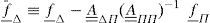
This algorithm is referred to as the ‘DVS-primal algorithm’. The solution is given by
We observe that we could have written u_;Δ=v_;Δ+S__−1f_;Δ instead of Eq. (5.6). However, the application of the projection operator a__ is important when ν_;Δ and S__−1f_;Δ are not computed with exact arithmetic, as it is the case when using numerical methods, because when it is applied it replaces v_;Δ+S__−1f_;Δ by the continuous-vector closest (with respect to the Euclidean distance) to it.
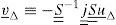
5.2Dual FormulationsThe DVS Version of FETI-DPFor this algorithm the sought-information is defined to be: λ_;Δ≡−j__S__u_;Δ. This algorithm can be easily derived from the DVS-primal formulation that has just been presented. We observe that v_;Δ=S_;−1λ_;Δ,λ_;Δ=S__ν_;Δ, in view of Eq. (5.2), and a__λ_;Δ=0. This permits transforming Eq. (5.5) into

Applying S__−1 to the first of these equations, it is obtained:

As for Eq. (5.6), it becomes:
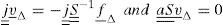
The DVS-Dual Algorithm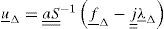
In this algorithm, the sought-information is: μ_;Δ≡S__u_;Δ. Then, u_;Δ=S__−1μ_;Δ. Replacing this in Eq. (5.1), one gets:

Finally, multiplying by S__ the first of these equalities, it is obtained:

When μ_;Δ is known, u_;Δ can be recovered by means of
A comment similar to that made immediately after Eq. (5.6), goes here: we have applied the projection matrix a__, in Eq. (5.12) because we are assuming that exact arithmetic generally will not be used.
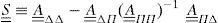
6Numerical Procedures Fulfilling the DDM-ParadigmSummarizing, the preconditioned DVS-algorithms with constraints are:
6.1Comment on the DVS Numerical Procedures


The outstanding uniformity of the formulas given in Eqs. (6.1) to (6.4) yields clear advantages for code development, especially when such codes are built using object-oriented programming techniques. Such advantages include:
- I.
The construction of very robust codes. This is an advantage of the DVS-algorithms, which stems from the fact the definitions of such algorithms exclusively depend on the discretized system of equations, obtained after discretization of the partial differential equations considered (referred to as the original problem), but which is otherwise independent of the problem that motivated it. In this manner, for example, essentially the same code was applied to treat 2-D and 3-D problems; indeed, only the part defining the geometry had to be changed, and that was a very small part of it;
- II.
The codes may use different local solvers, which can be direct or iterative solvers;
- III.
Minimal modifications are required for transforming sequential codes into parallel ones; and
- IV.
Such formulas also permit developing codes which fulfill the DDM-paradigm; i.e., in which “the solution of the global problem is obtained by exclusively solving local problems”.
This last property makes the DVS-algorithms very suitable as a tool to be used in the construction of massively-parallelized software, so much needed for efficiently programming the most powerful parallel computers available at present. In the next Subsection, procedures for constructing codes possessing Property IV are explained with some detail.
All the DVS-algorithms of Eqs. (6.1) to (6.4) are iterative and can be implemented with recourse to Conjugate Gradient Method (CGM), when the matrix is definite and symmetric, or some other iterative procedure such as GMRES, when that is not the case. At each iteration step, depending on the DVS-algorithm that is applied, one has to compute the action on a derived-vector of one of the following matrices: a__S__−1a__S__, j__S__j__S__−1, S__−1j__S__j__ or S__a__S__−1a__. Such matrices in turn are different permutations of the matrices S__, S__−1, a__ and J__. Thus, to implement any of the preconditioned DVS-algorithms, one only needs to separately develop codes capable of computing the action of each one of the matrices S__, S__−1, a__ or j__ on an arbitrary derived-vector, of W.
Therefore, next we present numerical procedures for computing the application of each one of the matrices S__, S__−1, a__ and j__ which fulfill the DDM-paradigm. It will be seen that only a__ requires exchange of information between derived-nodes belonging to different subdomains; actually, between derived-nodes that are descendants of the same original-node (the exchange of information is minimal). As for j__=I__−a__ once the action of a__ has been computed, no further exchange of information is required.
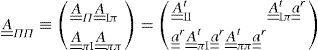
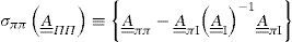
6.2Application of S__From Eq. (4.13), we recall the definition of the matrix S__≡A__ΔΔ−A__ΔΠA__ΠΠ−1A__ΠΔ. In order to evaluate the action of S__ on any derived-vector, we need to successively evaluate the action of the following matrices A__ΠΔ, A__ΠΠ−1, A__ΔΠ and A__ΔΔ. Nothing special is required except for A__ΠΠ−1. A procedure for evaluating the action of this matrix, which fulfills the DDM-paradigm is explained next.
We have
Let ν_;∈W, be an arbitrary derived-vector, and write
Then, w_;=w_;I+w_;π∈W is characterized by

and can obtained iteratively. Here,
and, with a__π as the projection-matrix into Wr(π),j__π≡I__−a__π.
We observe that fulfilling the DDM-paradigm when computing the action of A__II−1 is straightforward because
is parallelizable. Once v_;π∈Wr(π) has been obtained, to derive ν_;I one can apply:
this completes the evaluation of S__.
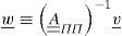
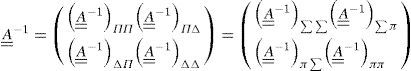
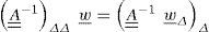
6.3Application of S__−1We define

and observe that

Therefore, the matrix A__−1 can be written as:
Furthermore, S__:WΔ→WΔ fulfills
Another property that is relevant for the following discussion is:
for any ν_;∈W, let us write

then, w_;π fulfills

Here, j__r≡I__−a__r, where the matrix a__r is the projection operator on Wr′ while
Furthermore, we observe that
In order to use Eq. (6.19) as a means of parallelizing the DVS-algorithms, however, the detailed discussion of such procedures will be presented separately [Herrera et al., 2013; L.M. de la Cruz et al., 2013]. It is necessary that the local matrices, A__∑∑α, be invertible. This is granted when invertible A__ in Wr′ which generally is achieved by taking a sufficiently large number of primal-nodes.
Eq. (6.17) is solved iteratively. Once ν_;π has been obtained, we apply:
This procedure permits obtaining A__−1w_; in full; however, we only need A__−1ΔΔw_;. We observe that
The vector A__−1w_;Δ can be obtained by the general procedure presented above. Thus, take w_;≡w_;Δ∈WΔ⊂W and
6.4Application of a__ and j__.

We use the notation

then [Herrera et al., 2010]:

while j__=I__−a__ therefore,

Therefore, only the evaluation of a__u_; requires exchange of information between subdomains. In general, such numbers are very small; for example in application to single-equation problem, when an orthogonal grid is used, they are at most: 4, for problems in 2D, and 8 for problems in 3D.
As for the right hand-sides of Eqs. (4.14), all they can be obtained by successively applying to f_;Δ some of the operators that have already been discussed. Recalling Eq. (4.14), we have
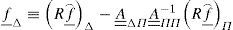
The computation of Rf⌢_; does not present any difficulty and the evaluation of the actions of A__ΠΠ−1 and A__ΔΠ were already analyzed.
7Numerical ResultsTaking into account the general description of the DVS-framework given of Section 2, it can be seen that each one of the DVS-algorithms is uniquely defined by:
- 1.
The original-matrix;
- 2.
The partition of the set of original-nodes, which is induced by the coarse-mesh that is applied; and
- 3.
The set of constraints.
In turn, the original-matrix is determined by the partial differential equation, or system of such equations, the discretization method chosen and the fine-mesh adopted. As explained in Section 2, the partition of the set of original-nodes depends when the fine-mesh has already been defined, on the coarse-mesh (i.e., the domain decomposition) used. The coarse-mesh is constituted by a family of non-overlapping subdomains {Ω1,..., ΩE} of Ω, the domain of definition of the boundary-value problem to be solved. In all the examples that are presented in this article, the constraints are fully determined by the primal-nodes and consist in requiring continuity of the derived-vectors at them.
Several codes were developed to treat the examples, which were written in C++ language, using the MPI library for the communications. In the computational implementations, the methods of solution used to treat the original-problems are: CGM, when such a linear system is symmetric and positive-definite and GMRES when the discrete system is non-symmetric or indefinite. Both are applied with a tolerance of 10−6. Each DVS-algorithm was applied to each one of the examples considered, except for that referring to elasticity.
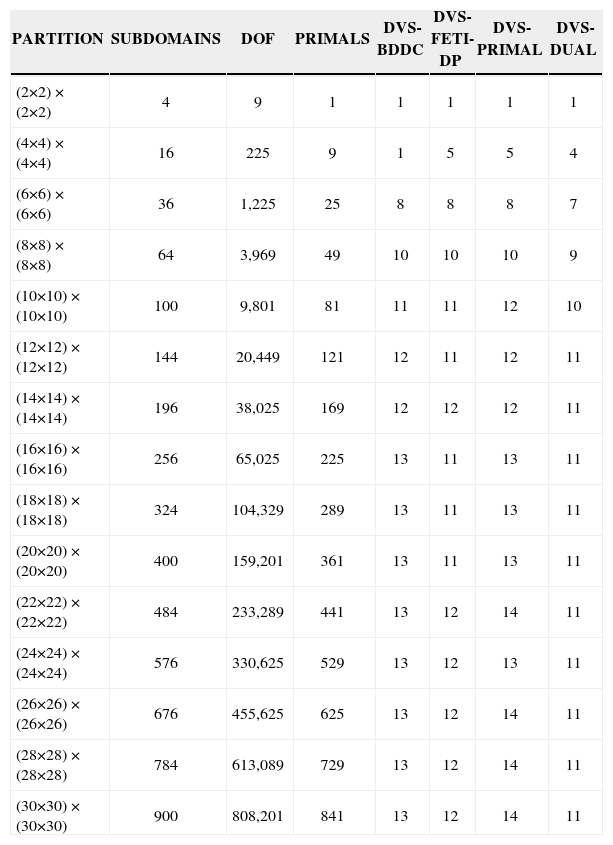
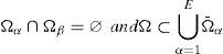
The results obtained for Examples 1 to 5 are summarized in Tables 1 to 5, respectively. In them, the acronym dof stands for to the number of degrees of freedom of the original problem, but it should be mentioned that the procedures used to treat such examples are such that the nodes that lie on the external boundary do not contribute to the dof. The notation to indicate the meshes that were adopted is as follows: In 2D cases, we use (nxm)x(qxr), where (nxm) refers to the coarsemesh, while (qxr) to the fine-mesh; and similarly, in 3D cases, we use (nxmxp)x(qxrxs), where (nxmxp) define the coarse-mesh and (qxrxs) the fine-mesh. The constrains are imposed on the primal nodes, in all of our experiments the primal nodes were located at vertex in 2D and at edges in 3D of the subdomains, this coinciding with the algorithm “D” in [Toselli et al., 2005].
Number of iterations made by the four DVS algorithms. The primal nodes were located at the vertices of subdomains.
| PARTITION | SUBDOMAINS | DOF | PRIMALS | DVS-BDDC | DVS-FETI-DP | DVS-PRIMAL | DVS-DUAL |
|---|---|---|---|---|---|---|---|
| (2×2) × (2×2) | 4 | 9 | 1 | 1 | 1 | 1 | 1 |
| (4×4) × (4×4) | 16 | 225 | 9 | 1 | 5 | 5 | 4 |
| (6×6) × (6×6) | 36 | 1,225 | 25 | 8 | 8 | 8 | 7 |
| (8×8) × (8×8) | 64 | 3,969 | 49 | 10 | 10 | 10 | 9 |
| (10×10) × (10×10) | 100 | 9,801 | 81 | 11 | 11 | 12 | 10 |
| (12×12) × (12×12) | 144 | 20,449 | 121 | 12 | 11 | 12 | 11 |
| (14×14) × (14×14) | 196 | 38,025 | 169 | 12 | 12 | 12 | 11 |
| (16×16) × (16×16) | 256 | 65,025 | 225 | 13 | 11 | 13 | 11 |
| (18×18) × (18×18) | 324 | 104,329 | 289 | 13 | 11 | 13 | 11 |
| (20×20) × (20×20) | 400 | 159,201 | 361 | 13 | 11 | 13 | 11 |
| (22×22) × (22×22) | 484 | 233,289 | 441 | 13 | 12 | 14 | 11 |
| (24×24) × (24×24) | 576 | 330,625 | 529 | 13 | 12 | 13 | 11 |
| (26×26) × (26×26) | 676 | 455,625 | 625 | 13 | 12 | 14 | 11 |
| (28×28) × (28×28) | 784 | 613,089 | 729 | 13 | 12 | 14 | 11 |
| (30×30) × (30×30) | 900 | 808,201 | 841 | 13 | 12 | 14 | 11 |
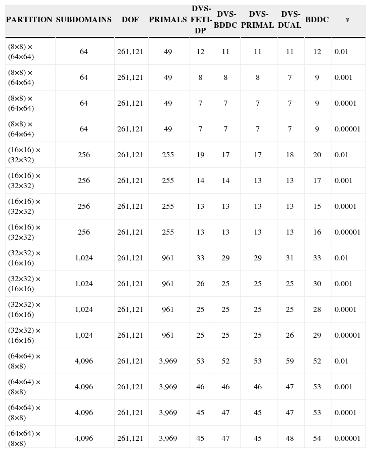
Each Table contains at most ten columns. The first four indicate respectively: 1) the meshes used, 2) the number of subdomains of the coarsemesh, 3) the dof, and 4) the number of primal-nodes used. The figures appearing in columns 5 to 9 correspond to the number of iterations that were required for convergence of each one of the algorithms applied. Columns 9 and 10 were only included in Table 3. For Example 3, in order to cover a wide range of values of the Peclet-number, the diffusion coefficient in Eq. (7.3), ν, was varied and the tenth column in Table 3 indicates the different values of ν for which the corresponding boundary-value problem was solved. Furthermore, the results obtained when the DVS-algorithms were applied were compared with those obtained in [Da Conceição et al., 2006] for the same problem, using the standard version of BDDC.
Comparison of the DVS-algorithms against the BDDC implemented in [Mandel et al., 1996].
| PARTITION | SUBDOMAINS | DOF | PRIMALS | DVS-FETI-DP | DVS-BDDC | DVS-PRIMAL | DVS-DUAL | BDDC | v |
|---|---|---|---|---|---|---|---|---|---|
| (8×8) × (64×64) | 64 | 261,121 | 49 | 12 | 11 | 11 | 11 | 12 | 0.01 |
| (8×8) × (64×64) | 64 | 261,121 | 49 | 8 | 8 | 8 | 7 | 9 | 0.001 |
| (8×8) × (64×64) | 64 | 261,121 | 49 | 7 | 7 | 7 | 7 | 9 | 0.0001 |
| (8×8) × (64×64) | 64 | 261,121 | 49 | 7 | 7 | 7 | 7 | 9 | 0.00001 |
| (16×16) × (32×32) | 256 | 261,121 | 255 | 19 | 17 | 17 | 18 | 20 | 0.01 |
| (16×16) × (32×32) | 256 | 261,121 | 255 | 14 | 14 | 13 | 13 | 17 | 0.001 |
| (16×16) × (32×32) | 256 | 261,121 | 255 | 13 | 13 | 13 | 13 | 15 | 0.0001 |
| (16×16) × (32×32) | 256 | 261,121 | 255 | 13 | 13 | 13 | 13 | 16 | 0.00001 |
| (32×32) × (16×16) | 1,024 | 261,121 | 961 | 33 | 29 | 29 | 31 | 33 | 0.01 |
| (32×32) × (16×16) | 1,024 | 261,121 | 961 | 26 | 25 | 25 | 25 | 30 | 0.001 |
| (32×32) × (16×16) | 1,024 | 261,121 | 961 | 25 | 25 | 25 | 25 | 28 | 0.0001 |
| (32×32) × (16×16) | 1,024 | 261,121 | 961 | 25 | 25 | 25 | 26 | 29 | 0.00001 |
| (64×64) × (8×8) | 4,096 | 261,121 | 3,969 | 53 | 52 | 53 | 59 | 52 | 0.01 |
| (64×64) × (8×8) | 4,096 | 261,121 | 3,969 | 46 | 46 | 46 | 47 | 53 | 0.001 |
| (64×64) × (8×8) | 4,096 | 261,121 | 3,969 | 45 | 47 | 45 | 47 | 53 | 0.0001 |
| (64×64) × (8×8) | 4,096 | 261,121 | 3,969 | 45 | 47 | 45 | 48 | 54 | 0.00001 |
The applicability of the DVS-algorithms is wide, as previously said it can be applied to general equation systems. In Section 3, it was n announced that in this paper we present examples for which d, the number of equation s of th e system, is one and three. In this Subsection the examples for which d=1 will be discussed, leaving for the next Subsection the treatment of static-elasticity models, for which d=3.
Four boundary value problems corresponding to a single-equation will be presented. The first two are symmetric and positive definite boundaryvalue problems, whose definition involves the Laplace differential operator. The other two correspond to advection-diffusion transport, and the corresponding boundary-value problems are non-symmetric and indefinite. The discretization methods used in this Subsection are based on central finite differences (CFD), which are directly applicable to the symmetric problems. To apply CFD to the advection-diffusion problems it was necessary to stabilize the advection-diffusion differential-operator and to this end artificial diffusion was incorporated.
Despite the simplicity of the examples presented in this Subsection, they are very important because a wide range of geophysical systems give rise to similar problems [Herrera and Pinder, 2012]. The diversity of physical interpretations of the boundary-value problems here discussed is enormous. All the differential operators involved can be classified as advection-diffusion operators, since Laplace operator is obtained from the general advection-diffusion differential-operator when the transport-velocity vanishes. Transport processes of heat and solutes occur in a great diversity of geophysical systems. However, the physical processes governed by such differential-equations go far beyond transport phenomena.
Example 1. Poisson equation in two-dimensions.

We can see from Table 1, that the four algorithms perform very well as the number of subdomains and the degrees of freedom (dof) are increased. In this example, the DVS-DUAL algorithm presents the best performance, requiring only 11 iterations from 12x12 until 30x30 subdomains, and the same number of dof. All other algorithms show similar behavior. The numerical solution of this example can be seen in the Figure 5.

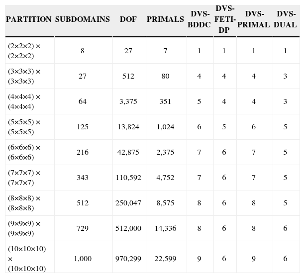
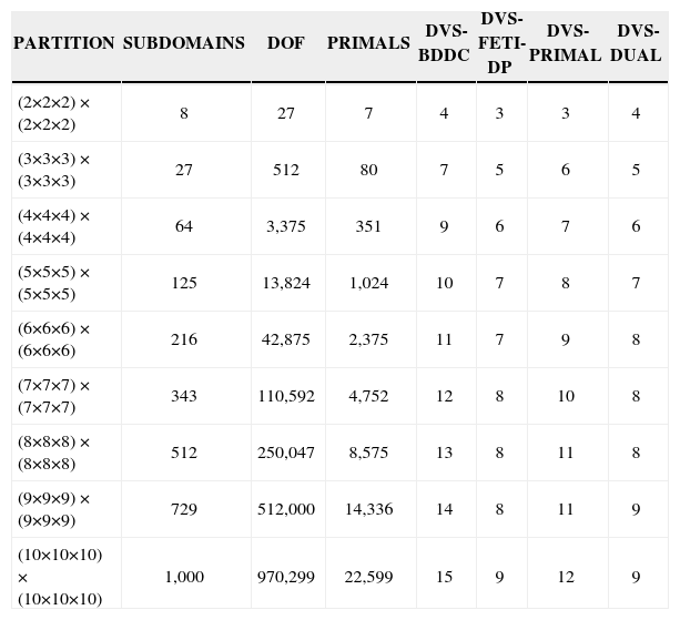
Example 2. Similar to Example 1, but it is formulated in a 3D domain.

In Table 2, we observe a similar performance of the algorithms as in the two-dimensional case. One more time the DVS-DUAL algorithm presents a little better behavior with respect all others.
Number of iterations made by the four DVS algorithms. The primal nodes were located at edge.
| PARTITION | SUBDOMAINS | DOF | PRIMALS | DVS-BDDC | DVS-FETI-DP | DVS-PRIMAL | DVS-DUAL |
|---|---|---|---|---|---|---|---|
| (2×2×2) × (2×2×2) | 8 | 27 | 7 | 1 | 1 | 1 | 1 |
| (3×3×3) × (3×3×3) | 27 | 512 | 80 | 4 | 4 | 4 | 3 |
| (4×4×4) × (4×4×4) | 64 | 3,375 | 351 | 5 | 4 | 4 | 3 |
| (5×5×5) × (5×5×5) | 125 | 13,824 | 1,024 | 6 | 5 | 6 | 5 |
| (6×6×6) × (6×6×6) | 216 | 42,875 | 2,375 | 7 | 6 | 7 | 5 |
| (7×7×7) × (7×7×7) | 343 | 110,592 | 4,752 | 7 | 6 | 7 | 5 |
| (8×8×8) × (8×8×8) | 512 | 250,047 | 8,575 | 8 | 6 | 8 | 5 |
| (9×9×9) × (9×9×9) | 729 | 512,000 | 14,336 | 8 | 6 | 8 | 6 |
| (10×10×10) × (10×10×10) | 1,000 | 970,299 | 22,599 | 9 | 6 | 9 | 6 |
Example 3. The boundary-value problem treated is:
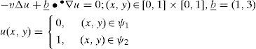
This is an advection-diffusion transport problem in 2D, for which the differential operator is not self-adjoint.
This example is very interesting because it contains diffusion and advection terms, which are common in several complex geophysics phenomena. In this example, the Péclet number is defined as Pe=b_;L/ν where L is a characteristic length (in this case L = 1). We also define a local Péclet number as Peh=b_;h/ν. Using these definitions, fixing the global partition to h=1/512, and the varying the viscosity from 0.01 to 0.0001, we have that the Péclet number varies from 316 to 316,227, and the local Péclet number varies from 0.617 to 617. In this case the linear system is non-symmetric, therefore we choose the GMRES method with a tolerance of 10−6.
In Table 3 presents the results that the DVS-algorithms yielded and compares them with those obtained in [Da Conceição et al., 2006]. We observe that, with fixed coarse and fine meshes, as the viscosity coefficient is reduced, so that the Péclet number increases, generally the iterations required for convergence reduce. Increasing the Péclet number implies that the effect of the advection term enlarges, and the numerical solution generally becomes unstable. However, the performance of the discretization strategy based on CFD combined with stabilization of the numerical-scheme by means of artificial viscosity is resilient to Péclet-number variations. For comparison purposes, the examples presented here were chosen to be the same as those presented in [Da Conceição et al., 2006], where the standard BDDC algorithm was applied with the same set of constraints; namely, the same set of subdomains and vertex nodes were chosen to be primal. As can be seen in Table 3, when the comparison criterion is based on the number of iterations required for convergence, the observed performance of the DVS-algorithms in these examples is slightly better than that of the standard BDDC algorithm. Finally, an illustration of the kind of numerical solution obtained is shown in Figure 7.


The relative-residual decay for a coarse mesh (16×16) and several fine meshes is presented in Figure 8. We consider in these computations b = (1, 3) and ν = 0.00001, in such a way that Pe = 3.16e+5. We observe that the best convergence is obtained when the fine mesh is increased, and the convergence slows when the dof occurring in the subdomains is reduced.
.")
Example 4. The boundary-value problem treated is:

This is an advection-diffusion transport problem in 3D, for which the differential operator is not self-adjoint.
The diffusion and advection-diffusion differential-operator appears in the equations of the examples presented above. They are very important in natural and industrial phenomena. For example, the flow and transport of solutes in subsurface groundwater, the movement of aerosol and trace gases in the atmosphere, mixing of fluids in processes of crystal growth, among many other important applications [Tood, 1980; Pinder et al., 2006; Herrera et al., 1969; Herrera et al., 1973; Herrera et al., 1977; Herrera G.S. et al., 2005; L.M. de la Cruz et al., 2006]. In all our examples, we have shown that the DVS-algorithms obtain the numerical solution efficiently on parallel machines. In this respect, we remark that for advection-diffusion problems the matrices of the discrete linear systems are non-symmetric.
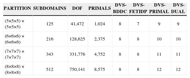
7.2Application to a System-EquationsWe use the DVS-framework to solve a Dirichlet boundary value problem, where displacements are zero over the boundary of the elastic body that occupies the domain Ω of the physical space. Over each one of such subdomains is solved a local problem by FEM, using linear functions as basis. On each node α of the mesh is defined a vector valued function u_;α with each component identified as uαi for i=1, 2, 3.
Number of iterations made by the four DVS algorithms. The primal nodes were located at edges of the subdomains.
| PARTITION | SUBDOMAINS | DOF | PRIMALS | DVS-BDDC | DVS-FETI-DP | DVS-PRIMAL | DVS-DUAL |
|---|---|---|---|---|---|---|---|
| (2×2×2) × (2×2×2) | 8 | 27 | 7 | 4 | 3 | 3 | 4 |
| (3×3×3) × (3×3×3) | 27 | 512 | 80 | 7 | 5 | 6 | 5 |
| (4×4×4) × (4×4×4) | 64 | 3,375 | 351 | 9 | 6 | 7 | 6 |
| (5×5×5) × (5×5×5) | 125 | 13,824 | 1,024 | 10 | 7 | 8 | 7 |
| (6×6×6) × (6×6×6) | 216 | 42,875 | 2,375 | 11 | 7 | 9 | 8 |
| (7×7×7) × (7×7×7) | 343 | 110,592 | 4,752 | 12 | 8 | 10 | 8 |
| (8×8×8) × (8×8×8) | 512 | 250,047 | 8,575 | 13 | 8 | 11 | 8 |
| (9×9×9) × (9×9×9) | 729 | 512,000 | 14,336 | 14 | 8 | 11 | 9 |
| (10×10×10) × (10×10×10) | 1,000 | 970,299 | 22,599 | 15 | 9 | 12 | 9 |
Because our operators are symmetric and positive definite, we use CGM as an iterative procedure to solve those linear systems of equations that we have defined in the DVS framework.
The code used in the previous section, which was originally developed to solve a single equation using finite differences, was adapted for solving systems of equations with FEM. We added the corresponding functionality in order to be able to solve systems of equations, in this case the elasticity problem.
Example 5. A system of partial differential equations in three-dimensions has also been treated. This is the system of differential equations of static elasticity; namely:

which was subject to the following Dirichlet boundary conditions:
The domain of study for our numerical experiments is a homogeneous isotropic linearly elastic unitary cube. In all of our experiments the primal nodes were located at edges of the subdomains, which is enough for A__t not being singular.
We consider constant coefficients λ and μ equal to one. With these conditions we have a problem that has analytical solution, and is written as follows:

The Tables 5, summarizes the numerical results obtained using the DVS methods with a tolerance of 10-7.
8ConclusionsMathematical models of many geophysical systems lead to a great variety of partial differential equations (PDEs) whose solution methods are based on the computational processing of largescale algebraic systems [Herrera and Pinder, 2012]. Parallel computing is outstanding among the new computational tools and, in order to effectively use the most advanced computers available today, massively parallel software is required. Domain decomposition methods (DDMs) have been developed precisely for effectively treating PDEs in parallel [DDM Organization, 2012]. What domain decomposition methods ideally intend to do has been summarized in this paper in the “DDM-paradigm”: to develop algorithms that ‘obtain the global solution by exclusively solving local problems’.
In conclusion, in this paper:
- 1.
We have presented a non-overlapping discretization method (the DVS-discretization) -in the sense that it uses a system of nodes such that each one of them belongs to one and only one subdomain of the coarse-mesh- applicable to a wide class of well-posed boundary problems associated with elliptic systems of equations. In particular, the differential operators may be symmetric, non-symmetric or indefinite (nonpositive-definite);
- 2.
Four algorithms –the DVS-algorithms [Herrera et al., 2011]-, which were derived using the DVS-discretization and achieve the DDM-paradigm have been explained. Two of them are the result of using the BDDC and FETI-DP algorithms after applying DVS-discretization to the boundary value problem considered. The other two are obtained when two new algorithms, which had not been reported previously in the literature, were used instead;
- 3.
Numerical procedures that permit achieving the DDM-paradigm with each one of the DVS-algorithms have been also presented;
- 4.
Codes were developed and applied to several boundary values problems that occur in the modeling of certain geophysical phenomena, such as transport of solutes by both, free-fluids and fluids in a porous medium. We also present results for a static elasticity problem, which thereby illustrates the application of the algorithms to systems of differential equations; and
- 5.
Besides their attractive parallelization properties, in the numerical examples the DVS-algorithms exhibited significantly improved numerical performance with respect to standard versions of BDDC and FETI-DP.
The authors express their gratitude to Alberto Rosas-Medina e Iván Contreras-Trejo, both PhD students of the Earth-Sciences Graduate Program at UNAM, for having permitted us to reproduce some numerical results of their research work.
Luis M. de la Cruz wishes to acknowledge the support from the project PAPIIT-UNAM TB100112 to develop this research.