


This paper presents a novel current transformer (CT) saturation detection approach based on Gaussian Mixture Models (GMMs). High accuracy is the advantage of this method. GMMs are trained with secondary current of CT. The appropriate performance of the proposed method is tested by simulation of different fault conditions in PSCAD/EMTDC software. The results show that the trained GMMs can successfully detect CT saturation with high accuracy.
Current transformer (CT) saturation distorts the secondary current and in consequence leads to operating delay or malfunction of protection relays (e. g. under reaching of over current relays, overestimation of fault loop impedance in distance relays) [1]. Therefore an appropriate saturation detection method is necessary to maintain the protection system reliability.
A method for detecting CT saturation onset based on the abrupt change in the current when CT saturates is suggested in [2]. This method can detect the saturation successfully only if the current collapses to zero after inception of saturation; however, it may operate incorrectly when the current does not change instantly when an anti-aliasing low-pass filter is used.
In [3], an algorithm for calculating the core flux from the secondary current in order to compensate the saturation is proposed. This algorithm calculates the core flux and detects saturation based on given CT parameters.
Another approach proposed in [4] is based on evaluating the mean of the error and the mean and variance of the current magnitude. The error is derived on the following assumption: If the currentis a perfect sinusoid, the summation of the current and its second-order derivative is zero over time. In [5] an impedance-based CT saturation detection algorithm for bus-bar differential protection is suggested. Calculation of power system source impedance at the relay position is based on a first-order differential equation. This method uses voltage and current signals of the bus-bar to detect CT saturation.
Another CT saturation detection algorithm based on the third difference of the secondary current is proposed in [6]. The effects of remanence flux in the core and a low-pass filter on the saturation are included in this method.
A method based on symmetrical components is suggested in [7]. The zero-sequence differential current gradient with respect to a bias current is utilized to detect saturation in a numerical current differential feeder protection relay.
Another approach for detecting CT saturation is the use of artificial intelligence (AI) techniques such as artificial neural networks (ANNs) (e.g., [8]). In [9], it is proved that considerable improvement of the operation and quite simple achievement of adaptive features of protection function may be obtained by utilizing various AI techniques [1]. Neural computing methodologies have some advantages over conventional methods. However there are no general rules for choosing the type of ANN structure and its further parameters (such as number of layers and neurons, neuron activation function, and input signals) which depend on designer experiences with ANN usage. To overcome this drawback, in [1] an optimization approach based on the genetic algorithm is proposed.
GMMs have been used as classifiers in a lot of applications such as speaker identification (SI) [10], multiple limb motion classification [11], image processing and classification [12,13], control engineering [14], simplification of controller design [15], and rotating machinery fault diagnosis [16]. In [17] wavelet based GMMs are used for magnetizing inrush current Identification. Recently, a time-domain analyzer based on GMMs has been introduced to discriminate permanent and transient faults [18].
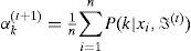
The ability of GMMs to solve nonlinear and high dimensional pattern problems makes them an appropriate choice in power system transient classifications [19]. In this paper, a new approach for CT saturation detection using GMMs is presented. Two GMMs are trained with the secondary current of CT. One of them is trained with CT secondary current when the fault inception angle is between 0–90 degrees and the other one is trained when the fault inception angle is between 90-180 degrees. This method of training GMMs for different fault inception angle improves the accuracy of the algorithm.
2Gaussian Mixture ModelsThe mathematical formulation of GMM is presented in this section [17].
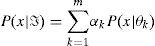
2.1DefinitionMixture models are types of probabilistic density models that comprise a number of component functions. These component functions, which are usually, Gaussian are combined to provide a multimodal density. These models are semi-parametric alternatives to nonparametric histograms (which can also be used as densities) and provide better flexibility and precision in modeling the underlying statistics of sample data. For an S-class pattern recognition system, a set of GMMs {ℑ1, ℑ2,...,ℑ3} are associated with S classes. A random variable x with D-dimensions is said to follow a Gaussian mixture model, when its probability density function can be formulated by Equation 1 following the constraints presented in Equation 2.
where αkis the mixture weight for the kth component, ℑ={α1,...,αm, μ1,...,μm, Σ1,...,Σm} is the complete set of parameters to define the model, and θk={μk,Σk} is the mean and covariance of the kth component, respectively. The Gaussian mixture density is a weighted linear combination of m component Gaussian density functions, θ1, θ2,..., θm. Each component density is a D-variant Gaussian function parameterized by a D×1 mean vector and a D×D covariance matrix. The component’s density P(x|θk) is a normal probability distribution defined by Equation 3:
2.2Training Process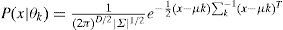
The goal of model training in a GMM-based classification system is to estimate the parameters of the GMM, ℑg so that the Gaussian mixture density can best match the distribution of the training feature vectors. For a set of n independent and identically distributed vectors X={x1, x2,... xn}, the corresponding likelihood of a mixture is
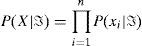
where P is the likelihood of the data X given the distribution parameters of ℑ. Specifically, by having the distribution parameters in ℑ, the goal is to find ℑ⌢ that maximizes the following likelihood:
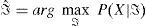
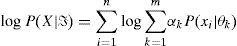
Usually, direct maximization of this function is difficult. The logarithm of the above probability, which is called the log-likelihood function given by Equation 6, is easier to calculate.
The logarithm of maximum likelihood estimation of each model ℑ cannot be solved analytically. The expectation maximization (EM) algorithm presented in [19] is widely used to estimate the parameters of GMM. EM is an iterative algorithm which maximizes the likelihood probability generated by each GMM, P (X | ℑg), given the data for that class. The EM algorithm has two main steps:
2.2.1E-stepIn this step, the posterior probability of sample xi in the tth step is calculated using the following equation:
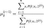
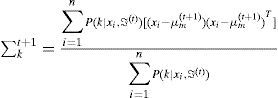
2.2.2M-step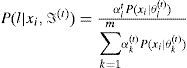
This re-estimation process will continue by replacing ℑˆ(t+1)={α1(t+1),…,αm(t+1),μ1(t+1),…,μm(t+1),∑1(t+1),…∑m(t+1)} instead of ℑ(t)={α1(t),…,αm(t),μ1(t),…,μm(t),∑1(t),…∑m(t)},, by using the following equations:
The above-mentioned method is discussed in more details in [20]. It should be noted that it is preferred to assume the S GMMs independent in calculations. In the case of independent classes, the estimation problem of S class pdfs can be divided into S separate estimation problems.
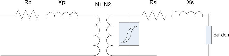
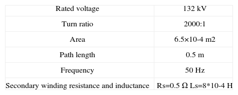
3Implementation Details3.1CT ModelA 132 kV power system including a CT is simulated to study CT saturation. The modeled CT is based on the Jiles-Atherton theory of ferro magnetic hysteresis [21]. In this model, the effects of saturation, hysteresis, remanence, and minor loop formation are modeled on the basis of the physics of the magnetic material [22]. In [23], the accuracy of this model has been checked. In [24], ANN is used to enhance the accuracy of this model. This model has been previously used to study the CT saturation compensation in [25].
In this model, the total magnetization (M) has been split in to two components [26]:
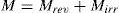
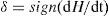
where Mrev and Mirr are reversible and irreversible magnetization components, respectively. Mirr is described as follows:
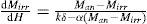
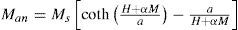
where δ is a directional parameter to distinguish between the ascending and the descending part of the hysteresis loop and Man is the unhysteretic magnetization provided by the Langevin function.
Finally, Mrev is given by
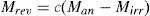
Among the five parameters of the JA model, Ms and a are the parameters of the unhysteretic curve which determine the saturation behavior of the magnetic core according to the Langevin function. The simulated CT in the present study is similar to the model used in [25], with the exception of the rated voltage, which is 132 KV in the present study. The model of the used CT is shown inFigure 1. Also, the parameters of the simulated CT are given in Table 1.
3.2Training Patterns
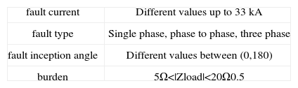
The training data set of a GMM should contain the information needed to generalize the problem. For this purpose, different fault types with different fault conditions are modeled using an EMTDC electromagnetic transient program [22]. A simple 132 kV power system is considered and several simulations for generating training patterns are done by changing fault current, fault type, fault inception angle, and burden. A combination of different fault conditions is shown in Table 2.
The saturation of CT is confirmed when the relative difference between the primary current i1' (related to the secondary) and the secondary current i2 is higher than 10% of the primary current [1]. Therefore, the time dependant training function for detecting the saturation is defined as follows:
3.3GMM Classification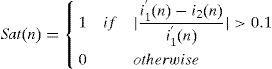
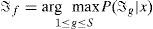
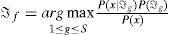
In this stage, the objective is to find the model which has the maximum probability Pmax for a given observation sequence. The test patterns are provided for each of the GMM models (Pℑ1,Pℑ2,..., PℑS), and S probabilities are computed and compared, i.e. Pi, i=1,2,...,S. Class f associated with the GMM that has the highest Gaussian mixture likelihood probability Pmax is chosen as the predicted class for the given feature set. A feature vector x produced by one type of signals (saturated or unsaturated secondary current of CT) is assumed. The identity of the signal is determined by finding signal model ℑf from S models which maximizes the probabilities across the signal set ℑg : g ∈ (1, S):
By using the Bayes rule, Equation 17 can be expressed as
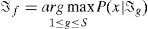
By assuming equal probabilities for all models and noting that P(x) is the same for them, the identification task can be summarized as finding the logarithm of the following equation:
Equation 19 can be expressed as the following equation for simplicity.
where αkg and θkg are mixture weight, mean, and covariance of the gth signal model, respectively.
3.4GMM ParametersIn order to achieve better performance of the Gaussian mixture model, an effort to investigate an optimum configuration of algorithmic issues must be considered [11]. These issues include convergence threshold, model order selection, and the form of the covariance matrix.
Convergence threshold of the EM Algorithm: The convergence threshold of the EM algorithm is defined as the difference between probabilities P(X | ℑg) between two consecutive iterations. The convergence threshold and the maximum iteration number are two conditions for stopping the EM algorithm. Different values of the convergence threshold were carefully examined and a value of 0.0005 was found to be the best for achieving good performance.
GMM Model Order: The GMM order selection is the most crucial factor in the performance of this classifier [11]. The objective is to choose the number of mixture components that yields the highest discriminative accuracy for the test data set. Theoretically, too few mixture components can yield a GMM which does not accurately model the distinguishing characteristics of classes. However, too many components can also reduce the performance, while increase the computation burden. It also makes the classification more complex. This is especially important for situations with smaller amounts of training data [11]. A larger model order should be considered when larger amounts of training data are available. Therefore, the optimal number of mixture components for the GMM must be carefully examined to achieve high classification performance. The optimal number of mixture is achieved by computing the classification rate presented in Equation 21 for test data set and varying the number of mixtures.

Form of the covariance matrix: Another effective issue on the performance of the classifier is the form of the covariance matrix. The form of the covariance matrix may be full or diagonal. In this work, diagonal covariance matrices are selected. This choice is based on empirical evidence that shows that diagonal matrices outperform full matrices. The diagonal matrix GMMs are more computationally efficient than full covariance GMMs for training since repeated inversions of a D×D matrix are not required [11].
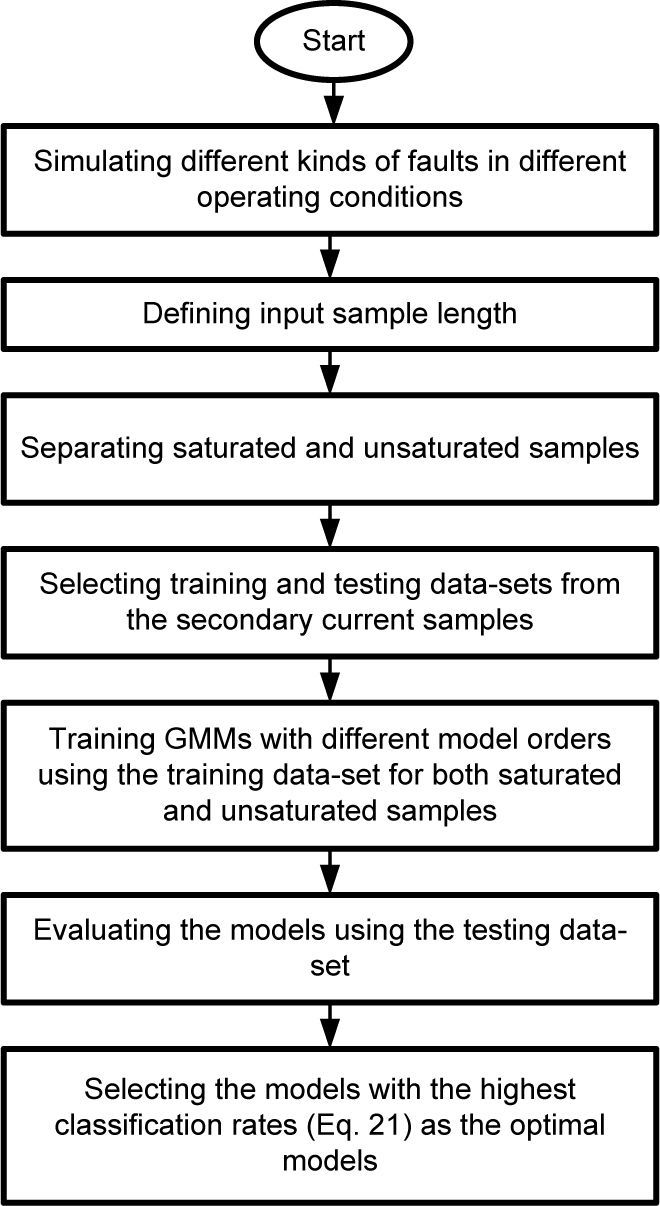
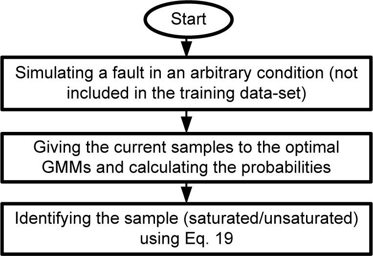
In the saturation detection problem, two GMMs should be trained. One for saturated and the other for unsaturated secondary current signals. The process of finding optimal GMMs is shown in the flowchart in Figure 2. After these two GMMs are found, the identification process for a new signal is as presented in the flowchart in Figure 3.
4Simulation Results

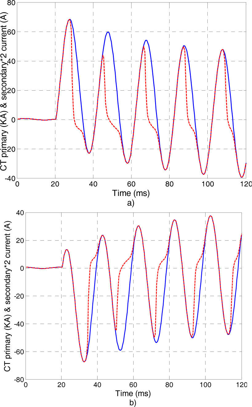
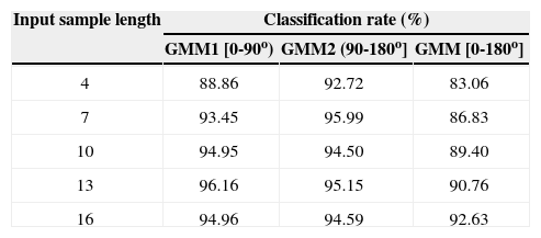
In this section, the training and testing process of GMMs for CT saturation detection is presented. As said in the previous section, a few hundred simulations have been performed. 70% of them are used for training and the remaining 30% are used for testing. Fault inception angles within [0,180] are considered in this study and two GMMs are trained. One of them for detecting the saturation when fault inception angle is between 0-90 degrees, and the other one for fault inception angles between 90-180 degrees. Fault inception angles between 180-360 degrees are not considered because of similarity. When a fault occurs, a switch can easily select one of the GMMs according to the fault inception angle. Training multiple GMMs for different fault inception angle ranges improves the accuracy of the method. Moreover, it does not need additional equipment or additional computation time. The primary and secondary currents of the used CT for fault inception angles equal to 45 and 135 degrees are illustrated in Figure 4(a) and Figure 4(b), respectively.
 45 degrees and b) 135 degrees.")
As can be seen in Figure 4, the wave forms of the CT for these cases have a great difference; therefore, training only one GMM for all of inception angle deteriorates the accuracy of the method.
The implementation results are presented in Table 3 for various numbers of input samples. To show the advantage of using two GMMs, the results of using only one GMM for all inception angles within [0,180] is also presented in this table.
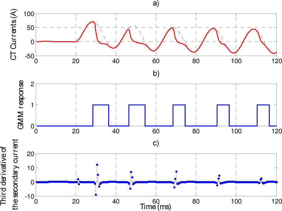
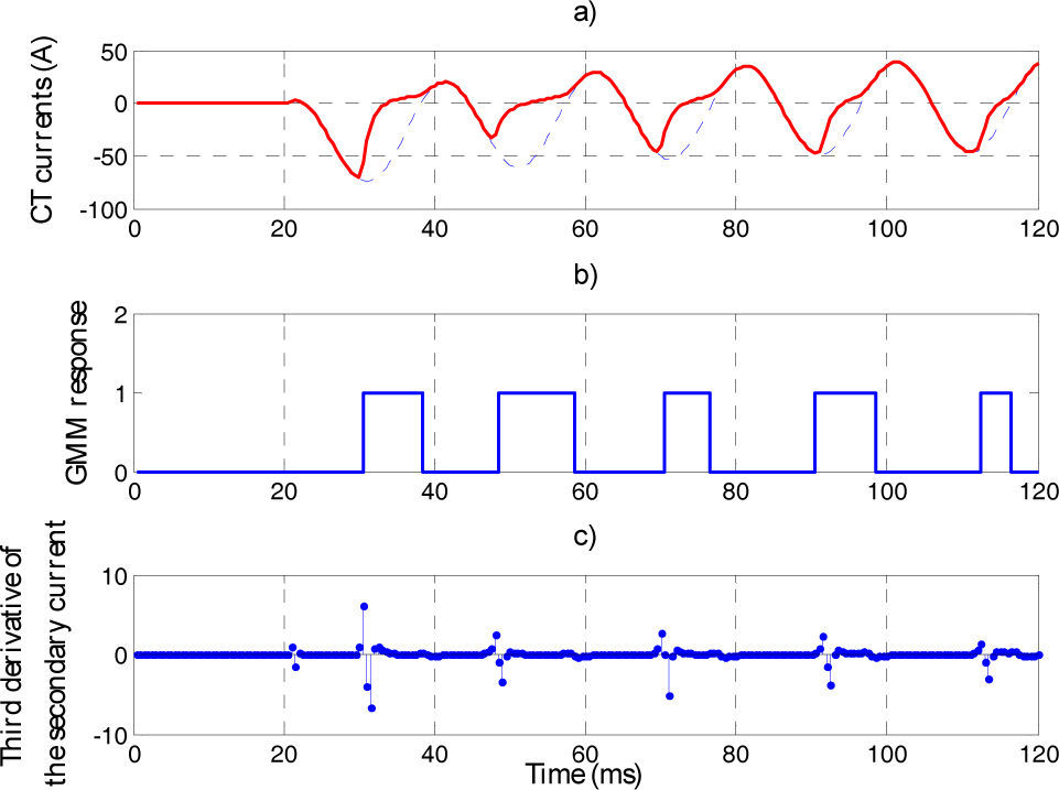
To show the ability of the proposed method to detect saturation in new situations (which were not included in the prepared data set), the trained GMM responses for two new cases are illustrated in Figures 5 and 6. Additionally, two examples of comparison between the developed GMM-based saturation detector and a chosen deterministic CT saturation identification scheme based on the calculation of the third derivative of the CT secondary current [27] are shown in these figures.
 CT signals, b) GMM1 response, c) third derivative of the secondary current.")
 CT signals, b) GMM1 response, c) third derivative of the secondary current.")
Figures 5 and 6 show that by using GMMs all starting and ending points of CT saturation intervals are properly detected. As can be seen in these figures, the third derivative shows high spikes at the beginning of the saturation, but there are no such spikes at the end of the saturation. Hence, this method detects the starting moments of the saturation properly but may have problems in detecting saturation endings.
5ConclusionA new approach for detecting CT saturation is presented in this paper which is based on a classification method called GMM. Secondary current samples are separated in two classes as saturated and unsaturated. GMMs are trained with the secondary current of CT in different conditions. To improve the accuracy of the method, two different GMMs are trained for fault inception angles between 0-90 degrees, and 90-180 degrees. Simulations are performed to confirm the effectiveness of the proposed GMM-based saturation detector. The results show that the proposed method can successfully detect the starting and ending points of saturation.