Food price inflation in India: The growing economy with sluggish agriculture

Abstract

India is experiencing high rate of economic growth in the last two decades but the growth has been coupled with high rate of food price inflation. The growth has been very uneven across sectors with agriculture remaining very sluggish. The increase in per capita income has significantly increased the demand for food but agricultural production has failed to keep pace with the growing demand. The theoretical explanations and time series econometric results establish that increase in per capita income and shortage in supply are responsible for price rise. There is no long run relationship between money supply and agricultural price. Increasing public expenditure and unfavorable foreign exchange rate have some effects on price although the results are not robust.

Resumen

India está experimentando un elevado índice de crecimiento económico en las últimas dos décadas, aunque dicho crecimiento ha ido acompañado de una elevada tasa de inflación de los precios de los alimentos. Este aumento se mostró bastante desigual entre los diferentes sectores, siendo muy lento en el sector agrícola. El incremento de la renta per cápita ha elevado considerablemente la demanda de alimentos, pero la producción agrícola no ha seguido el ritmo del crecimiento de la demanda. Las explicaciones teóricas y los resultados econométricos de las series de tiempo establecen que el incremento de la renta per cápita y la escasez de los suministros son los causantes del alza en los precios. No existe una relación a largo plazo entre el suministro dinerario y los precios agrícolas. El aumento del gasto público y las tasas poco favorables del cambio de divisas tienen ciertos efectos sobre los precios, aunque los resultados no son sólidos.

1

Introduction

India is experiencing high rate of GDP growth in the last two decades although the growth remains very uneven across sectors. The GDP is growing at a rate of 7-9% on an average per annum, but in agriculture the annual average growth rate is only 1.5% during this period. The share of agriculture in GDP has declined to less than 15%, although more than 50% of the population of the country is still dependent on agriculture for their livelihood. Like in many other developing countries the economic growth in India has been coupled with high rate of inflation. A major economic challenge the country is facing in the recent years is high food price inflation. From January 2008 to July 2010, the food price inflation rate year-on-year basis was recorded 10.20% (Nair & Eapen, 2012). From October 2009 to March 2010 food price inflation announced every week hovered around 20% (Basu, 2011). The researchers have tried to explain this price rise in terms of various factors including the effect of food crisis in the international market in the recent time (Gulati & Saini, 2013; Basu, 2011; Nair & Eapen, 2012). The Study of Robles (2011) shows that there is evidence of positive transmission effects of international prices on domestic agricultural markets in Asian and Latin American countries. Similar view has been expressed by Carrasco and Mukhopadhyay (2012). Baltzer (2013) however, notes that not all countries are equally hit by global food crisis. He states that in several countries, domestic prices are largely unrelated to international prices and reflect purely local shocks such as harvest failures, political turmoil etc. This study also finds that there is a close relationship between international and domestic prices in Brazil and South Africa, but the price pass-through from international to domestic market in China and India is almost nil. The level of transmission of international prices to domestic prices depends on a country's dependence on imports of food items and the inputs used in agricultural production. But India's dependence on the imports of agricultural products is not high except certain items like edible oils, sugar and pulses. In fact, India is a net exporter of food grains for the last thirty years although India's dependence on the import of petroleum and petro products including fertilizers is really very high. The management food economy and government intervention into the market for food grains through procurement and public distribution to maintain stability of food prices is an important issue in the present context. A sizeable buffer stock of food grains is maintained in India through public procurement to iron out the price fluctuations arising out of seasonal and sudden supply shocks especially in the years of crop failure. But Basu (2011) has shown that, the release of food grains was inadequate in the time of price rise although the food reserve in the country was above normal limit. So, the management of food economy was not up to the mark.

Like the price of any other commodity, agricultural price is also a market outcome and demand and supply in the market play an important role in the determination of price. The market imperfection can create distortion in the functioning of the market and influence price by controlling supply. A typical agricultural marketing channel is: Farmer – Local assembler – Central wholesaler – Retailer – Consumer. The retail prices are determined nearly in a perfectly competitive market situation. However, a few traders dominate in the wholesale market both as buyers and sellers. They act as both oligopolists and oligopsonists at the bottleneck of the marketing process (Nicholls, 1955; Sasmal, 2003). In the study of Osborne (2005) in the context of Ethiopia it is found that there are general forms of imperfect competition among rural wholesale traders, although there is no conclusive evidence of imperfect competition among the traders in larger and more centrally located markets. Anyway, the market imperfection can influence the price temporarily but it cannot sustain price rise for a long period if there is no actual shortage. There may be seasonal variation also in the prices of agricultural commodities. According to Sarkar (1993), prices are low in harvest season and high in lean season. Therefore, it is finally the supply and demand which are the most important determinants of agricultural price. The supply is related to agricultural production. In sluggish agriculture in a country like India, the productivity is stagnant or increasing at a declining rate due to various reasons like resource degradation, decline in public investment and technological bottlenecks (Sasmal, 2012; Bhullar & Sidhu, 2006; Mani, Bhalachandran & Pandit, 2011). But the demand for food items is increasing at a very high rate following a steady increase in per capita income. Higher disposable income has not only significantly increased the overall demand for agricultural commodities but also changed the pattern of consumption. Gulati and Saini (2013) have shown that the pressure on prices is more on protein foods like pulses, milk and milk products, egg, fish and meat and vegetables indicating the shift in consumption pattern from cereal based diets to protein based diets due to rise in income. There has been nearly threefold increase of per capita income (at constant prices) in India in the last two decades and poverty has declined from 45% in 1993-94 to 22% in 2011-12 (Source: Planning Commission Government of India, 2013). The overall demand has been further magnified by huge public expenditure of the government on a number of welfare schemes like rural employment, food security of the poor, subsidies, pension and various allowances. A lion's share of this expenditure is spent on unproductive and less productive heads. This has increased demand significantly without making much contribution to supply. Naturally, there has been a mismatch between the growing demand and the actual production. The supply response studies in agriculture explain that just increase in price cannot raise production. Adequate infrastructure, proper technology and various supporting factors are necessary for higher production (Nerlove, 1958; Schultz, 1964; Mellor, 1966; Raj Krishna, 1963; Narain, 1965; Feder, 1980). Again, many of these facilities are of public good nature and they are provided by the government. But net public investment in agriculture has declined in India in the recent past (Mani et al., 2011). The Granger causality analysis in Gilbert (2010) has established the role of demand growth, monetary expansion and exchange rate movements in explaining price movements over time. The econometric results of Saghian, Reed and Merchant (2002), however, indicate that agricultural prices adjust faster than industrial prices to shocks in the supply of money affecting short run relative prices but long run neutrality of money does not hold.

The objective of this paper is to analyze the nature and extent of food inflation in India in the last two decades and investigate into the factors behind the price rise. The main query of this study is to see to what extent the growing demand for agricultural commodities in a booming economy with sluggish agriculture can explain the food price inflation in a country like India. The paper has been arranged as follows: Section I introduces the matter, Section II presents a theoretical framework for explaining the price rise of food grains in a two-sector general equilibrium model. Section III provides empirical evidences and econometric results. Section IV gives the summary and policy implications.

2

Theoretical framework

2.1

Agricultural price in a two-sector general equilibrium model

One important feature of agricultural price is that it exhibits sharp fluctuations over time compared to non-agricultural prices. This is because in agricultural production supply can not immediately adjust itself with the changes in demand. Moreover, the elasticity of demand for most of the agricultural products is so low that a small change in supply with demand remaining constant or a small change in demand with supply remaining unchanged causes a large change in price.

In this section, a theoretical framework of food price inflation has been constructed by using the framework of specific factor model of international trade developed by Jones (1971) and Jones and Marjit (2003) for explaining the price behavior in case of shortage in the agricultural market. Let us consider an economy with two production sectors —Agriculture and Non-Agriculture—. For simplicity, we may assume that agricultural sector produces only food grains and the production of food grains is denoted by X. The production of the Non-Agricultural sector is denoted by Y. The production of X depends on Land (T) and Labor (L) along with other factors like soil fertility, irrigation, public investment, technology and variable inputs which are treated as parameters. The supply of land is fixed and it is specific to agriculture. On the other hand, the production of Y depends on Capital (K), Labor (L) and a set of parameters consisting of technology, infrastructure, human skill and so on. K is fixed and specific to Y. L is mobile between sectors and it is used both in X and Y.

The production functions are:

The production functions follow constant returns to scale with diminishing returns. If more labor (L) is used with the fixed amount of land (T) there will be diminishing returns in the production of X. The same is true for Y.

There is full employment of factors:

where aTx and aKy are per unit requirements of T and K in the production of X and Y respectively.

The prices of X and Y are P_X and P_Y respectively and in competitive market equilibrium the prices are:

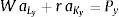
where, W, R and r are wage rate for labor, rental on land and rental on capital respectively. Labor is allocated between the two sectors following the condition:

Here, P_Y is numeriere and P=PXPY is relative price of X. So, VMP_L^X = P.MP_L^X and VMP_L^Y = MP_L^Y because P_Y/P_Y = 1.

The optimal allocation of labor between the two sectors and equilibrium wage rate are determined in Figure 1.

Figure 1.

Determination of optimal allocation of labor between two sectors and wage rate.

Author elaboration drawn on the basis of theoretical arguments of this paper.

The production of X and Y are determined as

If P rises L_x increases and this leads to increase in production of X. So, the relative supply of X (X/Y)^S is an increasing function P. Figure 1 shows that as P rises VMP_L^X curve shifts upward with the result that L_X increases.

The total income of the economy is PX + Y and fraction ∈ of this income is spent on X i.e.

where ∈ is the fraction of income.

After rearrangement, we get

Here, the relative demand for X, XYd inversely varies with P. We assume that demand is homothetic implying that goods ratio remains constant at all levels of income. The equilibrium P is determined in Figure 2. XYd and XYS curves may shift due to change in external factors causing change in P.

Figure 2.

Determination of equilibrium price (P).

Author elaboration drawn on the basis of theoretical arguments of this paper.

Let us now introduce money supply into the system and determine the nominal price of X, P_X. Suppose, there is a given supply of money denoted by M¯S and given velocity of circulation of money 1v. So, in equilibrium in the money market, we have

The equation (9) can be expressed as

It is further simplified to

and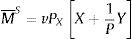

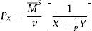
Here, P_X is determined in terms of X, Y, M^S and P. P_X is directly related with relative price (P) and money supply (M^S).

Let us now consider the relative change in X, Y, P and M ^S as Xˆ=dXX,Yˆ=dYY,Pˆ=dPP and MˆS=dMSMS.

The change in relative supply of X is:

The change in relative demand for X is:

where α is elasticity of relative supply with respect to P and β is elasticity of relative demand with respect to P. α_S and β_d are elasticity of relative supply and elasticity of relative demand respectively with respect to external factors. α_S and β_d depend on the factors other than price. The factors may be technology, public investment, income, preference, crop failure, external effects which are taken as parameters in the model.

In equilibrium

The equation (13) can be solved as

The elasticities of supply and demand of food items w.r.t. price are low. So, the values of α and β are low. Now, if elasticity of food grains production w.r.t. external factors (α_S) remains low and elasticity of demand for food grains w.r.t. external factors (β_d) becomes high, Pˆ will be positive and high.

More clearly, if (α + β) is low and (β_d − α_S) is positive and high, Pˆ will be positive, implying that relative price of food grains will increase. α and β are low by nature. α_S may be low due to lack of irrigation, decline of public investment, technological backwardness etc. On the other hand, β_d may be high due to internal and external factors, higher purchasing power, change of preference, etc.

From supply side, the relative changes may be conceived as

Xˆ=α1Pˆ,Yˆ=−α2Pˆ and Xˆ−Yˆ=α1+α2Pˆ=αPˆ

If the effects of external factors are taken into consideration in production, it becomes Xˆ−Yˆ=αPˆ+αS (refer to equation (11)).

To consider the change in money supply let us take the following equation:

Now, following Jones (1971), it can be written as

where λ is share of food grains production in national income and v is constant.

From equation (15) we get,

After using the expression Yˆ=−α2Pˆ and Xˆ−Yˆ=αPˆ, we may obtain

After rearrangement it becomes

and

Taking the value of Pˆ from (14) we get

In equation (16) if βd−αSα+β is positive and the value of λα is low, PˆX will be positive even if MˆS=0. That means, if demand for food items increases at a higher rate in a growing economy but agricultural production fails to grow at the same rate (β_d − α_S) will be positive and food price inflation will be there no matter whether money supply increases or not. In fact, increase in money supply is neither necessary nor sufficient for food price inflation in this model. If the first term of equation (16) is negative due to high value of either α_S or λ, Pˆ may be negative or zero despite the fact that MˆS〉0. In the whole process, β_d and α_S are very important.

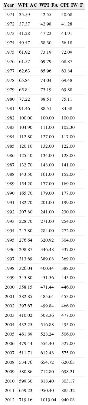
3

Empirical evidences and econometric results

3.1

Econometric results and discussion

This section gives the nature, trend and magnitude of food price inflation in India and makes econometric analysis using Time Series annual data to provide explanations for the increase of prices of food articles in the country. Table 1 and Figure 3 show that food inflation was moderate in India up to 1990 and after that the price index for food articles started rising sharply and from 2005 onward price rise has remained alarmingly high. It is indicated in Figure 3 that increase of wholesale price index for food articles (WPI_FA) was higher than the increase of consumer price index for food for industrial workers (CPI_WI_F). It is possibly because CPI_IW_F does not include many high value products like fruits, milk and meat, etc. that have shown tremendous price rise in recent years (see Nair & Eapen, 2012). It is interesting to note that food price inflation both in terms of WPI_FA and CPI_IW_F is much higher than general inflation denoted by the wholesale price index of all commodities (WPI_AC). While wholesale price index for all commodities (base 1981-82 = 100) has reached 719.16 in 2011-12, the index for food articles has risen to 1019.16 in the same period (see Table 1).

Table 1.

Price index of wholesale price for all commodities (WPI_AC), agricultural articles (WPI_FA) and consumer price index – Food grains for industrial workers (CPI_IW_F) in India with base on year 1981-82 = 100.

Year	WPI_AC	WPI_FA	CPI_IW_F
1971	35.59	42.55	40.68
1972	37.37	42.98	41.28
1973	41.28	47.23	44.91
1974	49.47	58.30	56.18
1975	61.92	73.19	72.09
1976	61.57	69.79	68.87
1977	62.63	65.96	63.84
1978	65.84	74.04	69.48
1979	65.84	73.19	69.88
1980	77.22	88.51	75.11
1981	91.46	88.51	84.38
1982	100.00	100.00	100.00
1983	104.90	111.00	102.30
1984	112.80	127.00	117.00
1985	120.10	132.00	122.00
1986	125.40	134.00	128.00
1987	132.70	148.00	141.00
1988	143.50	161.00	152.00
1989	154.20	177.00	169.00
1990	165.70	179.00	177.00
1991	182.70	201.00	199.00
1992	207.80	241.00	230.00
1993	228.70	271.00	254.00
1994	247.80	284.00	272.00
1995	276.64	320.92	304.00
1996	298.87	346.48	337.00
1997	313.69	389.08	369.00
1998	326.04	400.44	388.00
1999	345.80	451.56	445.00
2000	358.15	471.44	446.00
2001	382.85	485.64	453.00
2002	397.67	499.84	466.00
2003	410.02	508.36	477.00
2004	432.25	516.88	495.00
2005	461.89	528.24	506.00
2006	479.44	554.40	527.00
2007	511.71	612.48	575.00
2008	534.76	654.72	620.63
2009	580.86	712.80	698.21
2010	599.30	818.40	803.17
2011	659.23	950.40	885.32
2012	719.16	1019.04	940.08

Source: Economic Survey of India, 2012-13, Government of India and Handbook of Statistics on the Indian Economy, Reserve Bank of India.

Figure 3.

Trend of wholesale price index for all commodities (WPI_AC), food articles (WPI_FA) and consumer price index of food grains for industrial workers (CPI_IW_F).

Curves have been drawn by the author on the basis of data from Economic Survey, Government of India, 2000-01, 2012-13 and Handbook of Statistics on the Indian Economy, Reserve Bank of India, 2000-01, 2012-13.

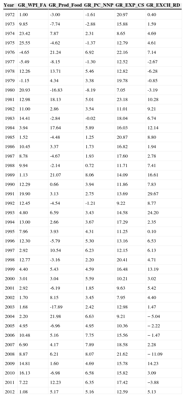
Table 2 shows annual growth rates of wholesale price index for food articles (GR_WPI_FA), production of food grains (GR_Prod_Food), per capita NNP at constant prices (GR_PC_NNP), public expenditure of the central and state governments (GR_EXP_CS) and Indian foreign-exchange rate with respect to US$ (GR_EXCH_RD). It indicates that annual price rise of food articles ranges from 6% to 16% for most of the time and prices remained continuously high over the period from 2005 to 2011. It is evident from Table 2 that the annual growth rate of food grains productions exhibits sharp fluctuations and in some years the growth rate has been found to be highly negative. In contrast, growth rate of per capita NNP (at constant prices) has remained consistently positive and high throughout the period since 1993. The growth rate of public expenditure of the central and state governments taken together is very high for the entire period. The growth rate of Indian foreign exchange rate (Indian Rupee per unit of US$) has shown fluctuations over the period although it shows positive trend for most of the time. It is interesting to note that during the period from 2004 to 2011, when agricultural price rise was very high, growth rate of exchange rate was negative. Figure 4 shows the growth rates of wholesale price index for food articles (GR_WPI_FA), per capita NNP at constant prices (GR_PC_NNP), production of food grains (GR_PROD_FOOD) and public expenditure of the Central and State governments (GR_EXP_CS).

Table 2.

Annual growth rates of wholesale price index of food articles (GR_WPI_FA), production of food grains (GR_PROD_FOOD), per capita NNP at constant price (GR_PC_NNP) and expenditure of Central and State Governments (combined) at current prices (GR_EXP_CS) and exchange rate of Indian Rupee with respect to US$ (GR_EXCH_RD).

Year	GR_WPI_FA	GR_Prod_Food	GR_PC_NNP	GR_EXP_CS	GR_EXCH_RD
1972	1.00	-3.00	-1.61	20.97	0.40
1973	9.85	-7.74	-2.88	15.88	1.59
1974	23.42	7.87	2.31	8.65	4.69
1975	25.55	-4.62	-1.37	12.79	4.61
1976	-4.65	21.24	6.92	22.16	7.14
1977	-5.49	-8.15	-1.30	12.52	-2.67
1978	12.26	13.71	5.46	12.82	-6.28
1979	-1.15	4.34	3.38	19.78	-0.85
1980	20.93	-16.83	-8.19	7.05	-3.19
1981	12.98	18.13	5.01	23.18	10.28
1982	11.00	2.86	3.54	11.01	9.21
1983	14.41	-2.84	-0.02	18.04	6.74
1984	3.94	17.64	5.89	16.03	12.14
1985	1.52	-4.48	1.25	20.87	8.80
1986	10.45	3.37	1.73	16.82	1.94
1987	8.78	-4.67	1.93	17.60	2.78
1988	9.94	-2.14	0.72	11.71	7.41
1989	1.13	21.07	8.06	14.09	16.61
1990	12.29	0.66	3.94	11.86	7.83
1991	19.90	3.13	2.75	13.69	29.67
1992	12.45	-4.54	-1.21	9.22	8.77
1993	4.80	6.59	3.43	14.58	24.20
1994	13.00	2.66	3.67	17.29	2.35
1995	7.96	3.93	4.31	11.25	0.10
1996	12.30	-5.79	5.30	13.16	6.53
1997	2.92	10.54	6.23	12.15	6.13
1998	12.77	-3.16	2.20	20.41	4.71
1999	4.40	5.43	4.59	16.48	13.19
2000	3.01	3.04	5.59	10.21	3.02
2001	2.92	-6.19	1.85	9.63	5.42
2002	1.70	8.15	3.45	7.95	4.40
2003	1.68	-17.89	2.42	12.98	1.47
2004	2.20	21.98	6.63	9.21	− 5.04
2005	4.95	-6.96	4.95	10.36	− 2.22
2006	10.48	5.16	7.75	15.56	− 1.47
2007	6.90	4.17	7.89	18.58	2.28
2008	8.87	6.21	8.07	21.62	− 11.09
2009	14.81	1.60	4.69	15.78	14.23
2010	16.13	-6.98	6.58	15.82	3.09
2011	7.22	12.23	6.35	17.42	−3.88
2012	1.08	5.17	5.16	12.59	5.13

Source: Calculated from the data in Economic Survey of India, 2012-13, Government of India and Handbook of Statistics on the Indian Economics, Reserve Bank of India, 2012-13.

Figure 4.

Growth rate of public expenditure (GR_EXP_CS), per capita NNP (GR_PC_NNP), food grains production (GR_PROD_FOOD) and wholesale price index for food articles (GR_WPI_FA).

Curves have been drawn by the author on the basis of data from Economic Survey, Government of India, 2000-01, 2012-13 and Handbook of Statistics on the Indian Economy, Reserve Bank of India, 2000-01, 2012-13.

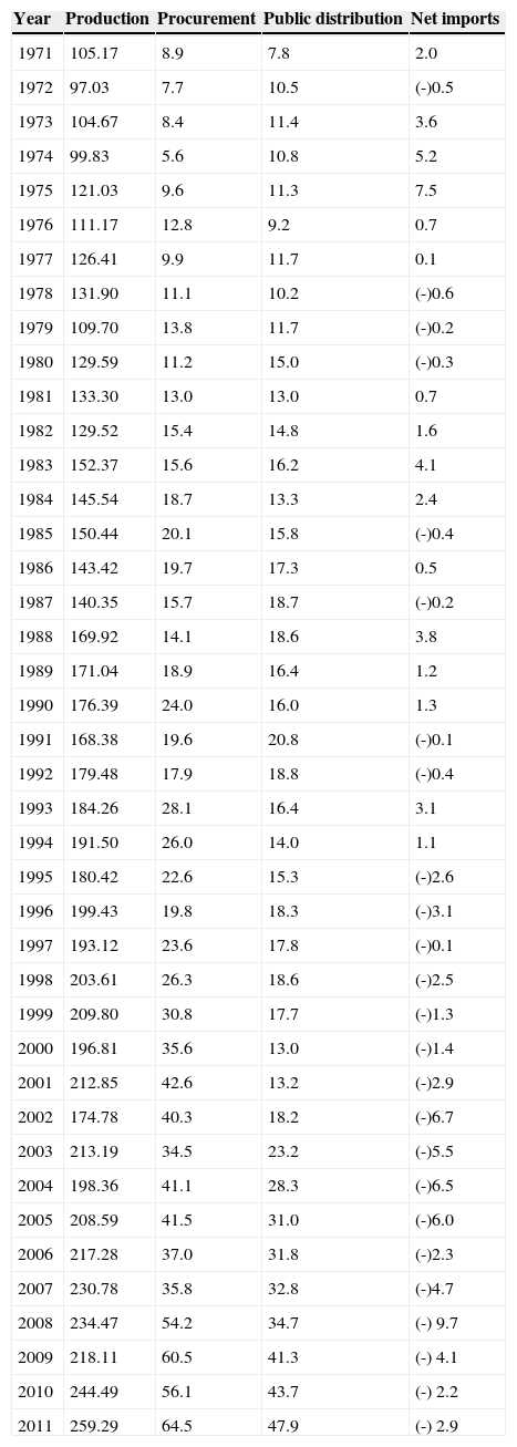
Table 3 shows total production, procurement, public distribution and net import of food grains in India during the period from 1971 to 2011. Both production and procurement have increased over time but the rate of procurement has remained higher than the rate of production. Again, the release of food grains through public distribution system remained lower than procurement. It indicates, government intervention could not be effective in stabilizing the prices of agricultural commodities. Table 3 also indicates that India is a net exporter of food grains for a long period. So, the argument that the effect of global food crisis has been transmitted into the Indian domestic market does not seem to be much convincing.

Table 3.

Production, procurement, public distribution and net import of food grains in India (million tonnes).

Year	Production	Procurement	Public distribution	Net imports
1971	105.17	8.9	7.8	2.0
1972	97.03	7.7	10.5	(-)0.5
1973	104.67	8.4	11.4	3.6
1974	99.83	5.6	10.8	5.2
1975	121.03	9.6	11.3	7.5
1976	111.17	12.8	9.2	0.7
1977	126.41	9.9	11.7	0.1
1978	131.90	11.1	10.2	(-)0.6
1979	109.70	13.8	11.7	(-)0.2
1980	129.59	11.2	15.0	(-)0.3
1981	133.30	13.0	13.0	0.7
1982	129.52	15.4	14.8	1.6
1983	152.37	15.6	16.2	4.1
1984	145.54	18.7	13.3	2.4
1985	150.44	20.1	15.8	(-)0.4
1986	143.42	19.7	17.3	0.5
1987	140.35	15.7	18.7	(-)0.2
1988	169.92	14.1	18.6	3.8
1989	171.04	18.9	16.4	1.2
1990	176.39	24.0	16.0	1.3
1991	168.38	19.6	20.8	(-)0.1
1992	179.48	17.9	18.8	(-)0.4
1993	184.26	28.1	16.4	3.1
1994	191.50	26.0	14.0	1.1
1995	180.42	22.6	15.3	(-)2.6
1996	199.43	19.8	18.3	(-)3.1
1997	193.12	23.6	17.8	(-)0.1
1998	203.61	26.3	18.6	(-)2.5
1999	209.80	30.8	17.7	(-)1.3
2000	196.81	35.6	13.0	(-)1.4
2001	212.85	42.6	13.2	(-)2.9
2002	174.78	40.3	18.2	(-)6.7
2003	213.19	34.5	23.2	(-)5.5
2004	198.36	41.1	28.3	(-)6.5
2005	208.59	41.5	31.0	(-)6.0
2006	217.28	37.0	31.8	(-)2.3
2007	230.78	35.8	32.8	(-)4.7
2008	234.47	54.2	34.7	(-) 9.7
2009	218.11	60.5	41.3	(-) 4.1
2010	244.49	56.1	43.7	(-) 2.2
2011	259.29	64.5	47.9	(-) 2.9

Source: Economic Survey of India, 2012-13, Government of India.

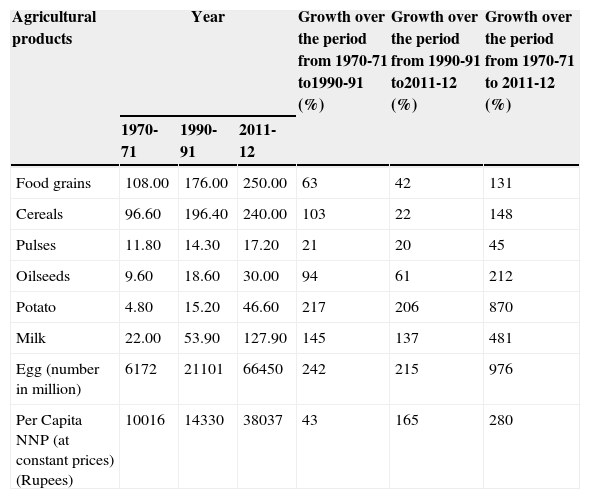
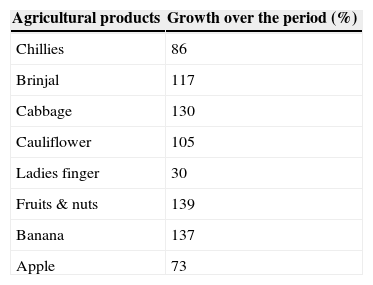
The information in Tables 4 and 5 is very revealing. They show that the growth rates in production of cereal and non-cereal agricultural items are much lower than the growth rate of per capita income (at constant prices). While the per capita NNP has increased by 165% during the period from 1990-91 to 2011-12, the growth rates of food grains, cereal, pulses and oilseeds are found to be much lower than the growth rate of per capita NNP. The growth rates of vegetables and fruits were also less than the growth rate of per capita income.

Table 4.

Production of food grains, cereal and some important non-cereal agricultural commodities in India (million tonnes).

Agricultural products	Year			Growth over the period from 1970-71 to1990-91 (%)	Growth over the period from 1990-91 to2011-12 (%)	Growth over the period from 1970-71 to 2011-12 (%)
	1970-71	1990-91	2011-12
Food grains	108.00	176.00	250.00	63	42	131
Cereals	96.60	196.40	240.00	103	22	148
Pulses	11.80	14.30	17.20	21	20	45
Oilseeds	9.60	18.60	30.00	94	61	212
Potato	4.80	15.20	46.60	217	206	870
Milk	22.00	53.90	127.90	145	137	481
Egg (number in million)	6172	21101	66450	242	215	976
Per Capita NNP (at constant prices) (Rupees)	10016	14330	38037	43	165	280

Source: Compiled from Economic Survey, 2012-13, Government of India.

Table 5.

Growth of production of vegetables and fruits in India (thousand tonnes) over the period from 1991-92 to 2008-09.

Agricultural products	Growth over the period (%)
Chillies	86
Brinjal	117
Cabbage	130
Cauliflower	105
Ladies finger	30
Fruits & nuts	139
Banana	137
Apple	73

Source: Centre for Monitoring Indian Economy (CMIE), June 2010.

3.2

Time series analysis

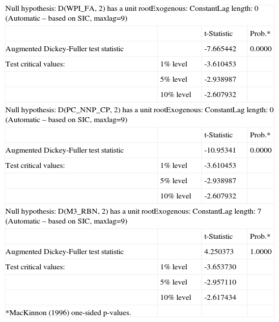
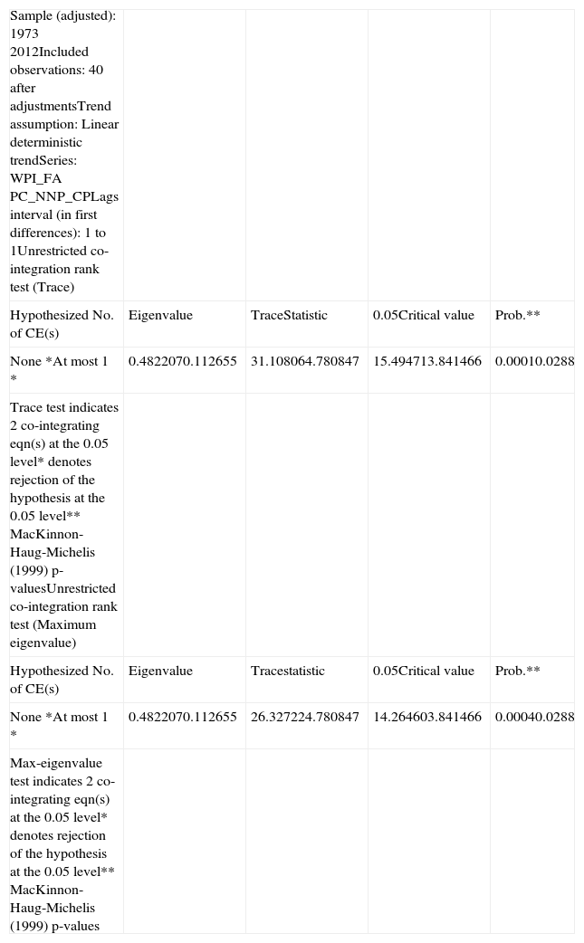
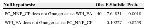
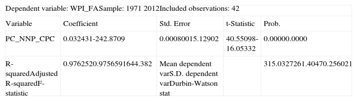
The stationarity of the series WPI_FA, GR_WPI_FA, PC_NNP_CP, money supply (M3_RBN), growth rate of production of food grains (GR_PROD_FOOD), growth rate of public expenditure (GR_EXP_CS) and growth rate of foreign exchange rate (GR_EXCH_RD) have been checked by using Augmented Dickey-Fuller Test. The results show that WPI_FA and PC_NNP_CP are stationary at 2nd difference. Money supply is non-stationary up to at 2nd difference (see Table 6a). In Johansen Co-integration Test WPI_FA and PC_NNP_CP are found to be co-integrated C(2,2) and in Granger Causality Test, the result shows that PC_NNP_CP causes WPI_FA (see Tables 6b and 6c). This is a very significant and strong result of this study. It establishes that there is meaningful long-run relationship between them and increase in per capita income is an important cause of price rise in the long-run. The regression results in Table 6d show that the adjusted R² is very high (0.97) and the coefficient is positive and highly statistically significant.

Table 6a.

Augmented Dickey-Fuller unit root test on D(WPI_FA, 2), D (PC_NNP_CP, 2) and D (M₃_RBN, 2).

Null hypothesis: D(WPI_FA, 2) has a unit rootExogenous: ConstantLag length: 0 (Automatic – based on SIC, maxlag=9)
		t-Statistic	Prob.*
Augmented Dickey-Fuller test statistic		-7.665442	0.0000
Test critical values:	1% level	-3.610453
	5% level	-2.938987
	10% level	-2.607932
Null hypothesis: D(PC_NNP_CP, 2) has a unit rootExogenous: ConstantLag length: 0 (Automatic – based on SIC, maxlag=9)
		t-Statistic	Prob.*
Augmented Dickey-Fuller test statistic		-10.95341	0.0000
Test critical values:	1% level	-3.610453
	5% level	-2.938987
	10% level	-2.607932
Null hypothesis: D(M3_RBN, 2) has a unit rootExogenous: ConstantLag length: 7 (Automatic – based on SIC, maxlag=9)
		t-Statistic	Prob.*
Augmented Dickey-Fuller test statistic		4.250373	1.0000
Test critical values:	1% level	-3.653730
	5% level	-2.957110
	10% level	-2.617434
*MacKinnon (1996) one-sided p-values.

Results have been obtained using the data from Economic Survey, Government of India, 2000-01, 2012-13 and Handbook of Statistics on the Indian Economy, Reserve Bank of India, 2000-01, 2012-13.

Table 6b.

Johansen co-integration test between WPI_FA and PC_NNP_CP.

Sample (adjusted): 1973 2012Included observations: 40 after adjustmentsTrend assumption: Linear deterministic trendSeries: WPI_FA PC_NNP_CPLags interval (in first differences): 1 to 1Unrestricted co-integration rank test (Trace)
Hypothesized No. of CE(s)	Eigenvalue	TraceStatistic	0.05Critical value	Prob.**
None *At most 1 *	0.4822070.112655	31.108064.780847	15.494713.841466	0.00010.0288
Trace test indicates 2 co-integrating eqn(s) at the 0.05 level* denotes rejection of the hypothesis at the 0.05 level** MacKinnon-Haug-Michelis (1999) p-valuesUnrestricted co-integration rank test (Maximum eigenvalue)
Hypothesized No. of CE(s)	Eigenvalue	Tracestatistic	0.05Critical value	Prob.**
None *At most 1 *	0.4822070.112655	26.327224.780847	14.264603.841466	0.00040.0288
Max-eigenvalue test indicates 2 co-integrating eqn(s) at the 0.05 level* denotes rejection of the hypothesis at the 0.05 level** MacKinnon-Haug-Michelis (1999) p-values

Results have been obtained using the data from Economic Survey, Government of India, 2000-01, 2012-13 and Handbook of Statistics on the Indian Economy, Reserve Bank of India, 2000-01, 2012-13.

Table 6c.

Pairwise Granger causality tests.

Null hypothesis:	Obs	F-Statistic	Prob.
PC_NNP_CP does not Granger cause WPI_FA	40	7.64831	0.0018
WPI_FA does not Granger cause PC_NNP_CP		0.19227	0.8259

Results have been obtained using the data from Economic Survey, Government of India, 2000-01, 2012-13 and Handbook of Statistics on the Indian Economy, Reserve Bank of India, 2000-01, 2012-13.

Table 6d.

OLS regression of WPI_FA on PC_NNP_CP.

Dependent variable: WPI_FASample: 1971 2012Included observations: 42
Variable	Coefficient	Std. Error	t-Statistic	Prob.
PC_NNP_CPC	0.032431-242.8709	0.00080015.12902	40.55098-16.05332	0.00000.0000
R-squaredAdjusted R-squaredF-statistic	0.9762520.9756591644.382	Mean dependent varS.D. dependent varDurbin-Watson stat		315.0327261.40470.256021

Results have been obtained using the data from Economic Survey, Government of India, 2000-01, 2012-13 and Handbook of Statistics on the Indian Economy, Reserve Bank of India, 2000-01, 2012-13.

On the other hand, money supply fails to explain the price rise. WPI_FA and M₃_RBN are not co-integrated implying that there is no meaningful long run relationship between them.

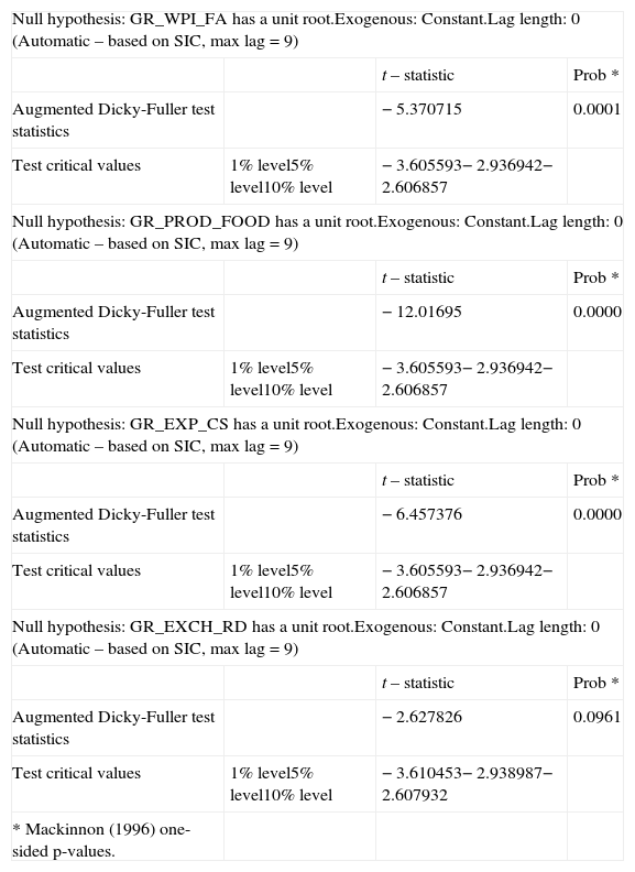
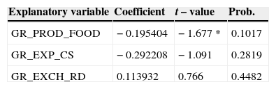
Since we are discussing food price inflation in a sluggish agriculture it is important to examine the relationship between growth rate of food grains production (GR_PROD_FOOD) and growth rate of prices of food articles (GR_WPI_FA). GR_WPI_FA and GR_PROD_FOOD are stationary at level and co-integrated in Johansen Test (see Tables 7a and 7b). The OLS estimation in Table 7e shows that there is statistically significant negative relationship between GR_PROD_FOOD and GR_WPI_FA. The significance of this result is that if supply of food grains declines due to crop failure or any other reasons, price rises. Figure 4 indicates that decline in the growth rate of food grains production is associated with sharp rise in the growth rate of food grains price.

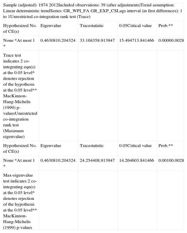
The other two important variables are growth rates of public expenditure of the Central and State governments (GR_EXP_CS) and Foreign exchange rate of Indian Rupee with respect to US$ (GR_EXCH_RD). It is theoretically argued that if public expenditure increases it will boost up demand leading to price rise. On the other hand, if the exchange rate (Rupees per unit of US$) rises it will increase the cost of imports putting an upward pressure on price. GR_EXP_CS, GR_EXCH_RD and GR_WPI_FA are stationary at level and they are co-integrated in Johansen Test although the results are not robust (see Tables 7a–7e). That means, public expenditure and foreign exchange rate have effects on agricultural prices but they are not very significant because there is no causality between them. The regression coefficients are also not significant (see Table 7e).

Table 7a.

Augmented Dicky-Fuller unit root test on GR_WPI_FA, GR_PROD_FOOD, GR_EXP_CS and GR_EXCH_RD.

Null hypothesis: GR_WPI_FA has a unit root.Exogenous: Constant.Lag length: 0 (Automatic – based on SIC, max lag = 9)
		t – statistic	Prob *
Augmented Dicky-Fuller test statistics		− 5.370715	0.0001
Test critical values	1% level5% level10% level	− 3.605593− 2.936942− 2.606857
Null hypothesis: GR_PROD_FOOD has a unit root.Exogenous: Constant.Lag length: 0 (Automatic – based on SIC, max lag = 9)
		t – statistic	Prob *
Augmented Dicky-Fuller test statistics		− 12.01695	0.0000
Test critical values	1% level5% level10% level	− 3.605593− 2.936942− 2.606857
Null hypothesis: GR_EXP_CS has a unit root.Exogenous: Constant.Lag length: 0 (Automatic – based on SIC, max lag = 9)
		t – statistic	Prob *
Augmented Dicky-Fuller test statistics		− 6.457376	0.0000
Test critical values	1% level5% level10% level	− 3.605593− 2.936942− 2.606857
Null hypothesis: GR_EXCH_RD has a unit root.Exogenous: Constant.Lag length: 0 (Automatic – based on SIC, max lag = 9)
		t – statistic	Prob *
Augmented Dicky-Fuller test statistics		− 2.627826	0.0961
Test critical values	1% level5% level10% level	− 3.610453− 2.938987− 2.607932
* Mackinnon (1996) one-sided p-values.

Results have been obtained using the data from Economic Survey, Government of India, 2000-01, 2012-13 and Handbook of Statistics on the Indian Economy, Reserve Bank of India, 2000-01, 2012-13.

Table 7b.

Johansen co-integration test between GR_WPI_FA and GR_PROD_FOOD.

Sample (adjusted): 1974 2012Included observations: 39 after adjustmentsTrend assumption: Linear deterministic trendSeries: GR_PROD_FOOD GR_WPI_FALags interval (in first differences): 1 to 1Unrestricted co-integration rank test (Trace)
Hypothesized No. of CE(s)	Eigenvalue	Tracestatistic	0.05Critical value	Prob.**
None *At most 1 *	0.5663140.368700	50.5209617.93902	15.494713.841466	0.00000.0000
Trace test indicates 2 co-integrating eqn(s) at the 0.05 level* denotes rejection of the hypothesis at the 0.05 level** MacKinnon-Haug-Michelis (1999) p-valuesUnrestricted co-integration rank test (Maximum eigenvalue)
Hypothesized No. of CE(s)	Eigenvalue	Tracestatistic	0.05Critical value	Prob.**
None *At most 1 *	0.5663140.368700	32.5819417.93902	14.264603.841466	0.00000.0000
Max-eigenvalue test indicates 2 co-integrating eqn(s) at the 0.05 level* denotes rejection of the hypothesis at the 0.05 level** MacKinnon-Haug-Michelis (1999) p-values

Results have been obtained using the data from Economic Survey, Government of India, 2000-01, 2012-13 and Handbook of Statistics on the Indian Economy, Reserve Bank of India, 2000-01, 2012-13.

Table 7c.

Johansen co-integration test between GR_WPI_FA and GR_EXP_CS.

Sample (adjusted): 1974 2012Included observations: 39 (after adjustments)Trend assumption: Linear deterministic trendSeries: GR_WPI_FA GR_EXP_CSLags interval (in first differences): 1 to 1Unrestricted co-integration rank test (Trace)
Hypothesized No. of CE(s)	Eigenvalue	Tracestatistic	0.05Critical value	Prob.**
None *At most 1 *	0.4630810.204324	33.168358.913947	15.494713.841466	0.00000.0028
Trace test indicates 2 co-integrating eqn(s) at the 0.05 level* denotes rejection of the hypothesis at the 0.05 level** MacKinnon-Haug-Michelis (1999) p-valuesUnrestricted co-integration rank test (Maximum eigenvalue)
Hypothesized No. of CE(s)	Eigenvalue	Tracestatistic	0.05Critical value	Prob.**
None *At most 1 *	0.4630810.204324	24.254408.913947	14.264603.841466	0.00100.0028
Max-eigenvalue test indicates 2 co-integrating eqn(s) at the 0.05 level* denotes rejection of the hypothesis at the 0.05 level** MacKinnon-Haug-Michelis (1999) p-values

Results have been obtained using the data from Economic Survey, Government of India, 2000-01, 2012-13 and Handbook of Statistics on the Indian Economy, Reserve Bank of India, 2000-01, 2012-13.

Table 7d.

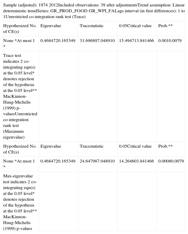
Johansen co-integration test between GR_WPI_FA and GR_EXCH_RD.

Sample (adjusted): 1974 2012Included observations: 39 after adjustmentsTrend assumption: Linear deterministic trendSeries: GR_PROD_FOOD GR_WPI_FALags interval (in first differences): 1 to 1Unrestricted co-integration rank test (Trace)
Hypothesized No. of CE(s)	Eigenvalue	Tracestatistic	0.05Critical value	Prob.**
None *At most 1 *	0.4684720.165349	31.696897.048910	15.494713.841466	0.0010.0079
Trace test indicates 2 co-integrating eqn(s) at the 0.05 level* denotes rejection of the hypothesis at the 0.05 level** MacKinnon-Haug-Michelis (1999) p-valuesUnrestricted co-integration rank test (Maximum eigenvalue)
Hypothesized No. of CE(s)	Eigenvalue	Tracestatistic	0.05Critical value	Prob.**
None *At most 1 *	0.4684720.165349	24.647987.048910	14.264603.841466	0.00080.0079
Max-eigenvalue test indicates 2 co-integrating eqn(s) at the 0.05 level* denotes rejection of the hypothesis at the 0.05 level** MacKinnon-Haug-Michelis (1999) p-values

Results have been obtained using the data from Economic Survey, Government of India, 2000-01, 2012-13 and Handbook of Statistics on the Indian Economy, Reserve Bank of India, 2000-01, 2012-13.

Table 7e.

OLS regression of GR_WPI_FA on GR_PROD_FOOD, GR_EXP_CS and GR_EXCH_RD.

Explanatory variable	Coefficient	t – value	Prob.
GR_PROD_FOOD	− 0.195404	− 1.677 *	0.1017
GR_EXP_CS	− 0.292208	− 1.091	0.2819
GR_EXCH_RD	0.113932	0.766	0.4482

Results have been obtained using the data from Economic Survey, Government of India, 2000-01, 2012-13 and Handbook of Statistics on the Indian Economy, Reserve Bank of India, 2000-01, 2012-13.

* significant at 10% level.

What finally comes out of this study is that it is the growth of per capita NNP that significantly explains the food price inflation in India. The sluggishness of agricultural production also accounts for the price rise. The market imperfection, government intervention and external trade do not seem to have any significant effect on food prices in the long run. Similarly, the effects of growing public expenditure and unfavorable foreign exchange rate are found to have some effects on agricultural price in the long run although the results are not very robust.

4

Political implications

4.1

Food price and the poor

Food price inflation has significant political implications. It reduces purchasing power and consumption level of the poor. Pinstrup-Anderson (1985) has found that low income consumers in developing countries typically spend 60-80% of their incomes on food and due to increase of food prices, real income decreases by 5.5% to 9% at the lowest decile. He has also shown that price elasticity of demand for rice for low income groups ranges from 1.23 to 4.31. Therefore, increasing food prices have serious welfare implications for the poor. Among the measures adopted by the government to give some relief and food security to the poor subsidy on food is an important one. The subsidy on food provides social safety net to the poor. The government of India allocates a hefty amount from the annual budget for procurement and distribution of food grains for this purpose. But the policy has now come under serious criticism because of its large contribution to budget deficit, economic inefficiency and poor targeting (Sharma, 2012). The subsidy on food in India has significantly increased in the post-reform period. In the years 2011-12, the amount of subsidy was Rupees 72,283 crore (Sharma, 2012) and in the annual budget of 2014-15, this amount has been raised to Rupees 1,15,000 crore (Reserve Bank of India Bulletin, 2014). But the problem is that a sizeable portion of this huge subsidy does not reach the target groups due to corruption, and lack of good governance and proper delivery mechanism. So, more effective policy measures are needed in this respect.

4.2

Public expenditure and food price inflation

The increase of public expenditure of the Central and State governments, though not very robust, has been found to be a cause of food price inflation in this study. The expenditure has increased at a rate of 10-20% per annum. But nearly 50% of this expenditure is spent on non-developmental purposes. More than 80% of the total expenditure of the Central government is spent on the heads of revenue expenditure that include salaries and wages, subsidies, pension and interest payment on loan. This huge expenditure increases demand in the market without contributing much to production. Sasmal (2011) demonstrates that if political gain from distributive expenses is higher, the government will have a tendency to spend more on such heads at the cost of long term growth. In fact, the government has a political compulsion in this matter. In India, National Rural Employment Guarantee Act (NREGA) has been passed and implemented to ensure employment to the jobless poor rural workers at statutory minimum wage rate and huge budgetary provisions are there for carrying out this scheme. In 2012-13 annual budget of the Central government financial allocation for NREGA is Rupees 90 000 crore which is more than 6% of the total budget. The problem with this scheme is that it does not help asset creation and production of the country to any significant extent although it boosts up demand in the market and puts huge financial burden on the government. As a result, the scheme has been brought under political controversy.

4.3

Agricultural growth and the role of the Government

The sectoral imbalance in GDP growth has serious consequences on the whole economy. Ray (2010) provides a framework for research in development economics in the context of uneven growth. India has achieved high rate of overall growth in the post-liberalization period largely banking on the expansion of the service sector which is growing at the rate of 10-12% per annum against less than 2% growth of the agricultural sector. The government has remained complacent with overall GDP growth and less attention has been given to the production sector. Especially agricultural has been grossly neglected by the government in the recent past. Overall growth and private investment in agriculture are conditional on public investment. Mani et al. (2011) have shown that real public investment in agriculture in India (in billion Rupees) has declined from 104.96 in the period 1979-80 to 1981-82 to 37.15 in 1999-2000. As a result, rate of annual investment in agriculture has gone down to 0.93% from 2.43% during this period. Now it has become imperative for the government to take appropriate measures to keep pace with the growing demand. Instead of dolling out money in the name of social security and welfare of the poor the government needs to allocate more funds for irrigation, agricultural research, technological innovations and resource management keeping in mind that government has a big role for agricultural growth in developing countries.

5

Summary and policy implications

India is experiencing high rate of GDP growth in the last two decades. But the growth has remained uneven across sectors and it has been associated with high rate of food price inflation. The demand for food articles has increased significantly with increase in per capita income over the years. But agricultural production has remained sluggish and failed to keep pace with the growing demand. The huge public expenditure of the government every year, mostly on unproductive or less productive heads has further magnified the demand. On the other hand, resource degradation, technological stagnation, lack of infrastructure and fall in public investment have created bottlenecks for increasing agricultural production. This paper has tried to analyze the trend and causes of food price inflation in India theoretically and with the help of econometric exercises.

A two-sector general equilibrium model has been constructed in the framework of specific factors trade model to demonstrate theoretically that if demand for agricultural commodities increases significantly due to increase of income and other external factors but supply fails to increase proportionately, agricultural prices will increase. In econometric exercise time series analyses have been done to verify the long run relationship between wholesale price index for agricultural commodities, per capita NNP and growth rate of food grains production. The effect of public expenditure, money supply and foreign exchange rate on agricultural prices has also been examined.

Empirical evidences suggest that food crisis in the global market in the recent years does not have much impact on India's domestic food price. The government intervention into the food grains market also fails to explain the phenomenon of price rise in the country. The time series analyses strongly establish that per capita income and wholesale price index for food articles are co-integrated and increase in per capita income has significant positive impact on food prices. The growth rate of food grains production is co-integrated with agricultural price index and a negative relationship between them has been obtained in the long run. This study finds no meaningful long run relationship between money supply and agricultural price. On the other hand, growing public expenditure and unfavorable foreign exchange rate are found to have impact on price although the results are not very robust.

Acknowledgement

The author expresses his thanks and gratitude to the anonymous Reviewer and the Editor of the Journal for the valuable comments on this paper. He also expresses his indebtedness to Professor Sugata Marjit for his help in writing this article. The help of Ritwik Sasmal is acknowledged. The usual disclaimer applies.