Editado por: Dr. Josep Arimany Manso - Colegi de Metges de Barcelona, Barcelona, Spain
Más datosForensic age assessment of living individuals has become a standard procedure in the field of legal medicine in many countries. The overall aim of forensic age assessment is to use the best available evidence for estimating the chronological age of an individual with dubious age information for legal purposes on behalf of courts or authorities. The scientific basis of forensic age assessment in adolescents and young adults is the predetermined temporal progression of defined stages of various developmental systems applicable to all individuals, such as skeletal maturation and dental development.1 The stage of development for a given age-related indicator is usually classified according to ordinal scale that has been pre-defined by forensic experts. The stage of an individual's development, rated according to this scale, is usually inferred from comparison to reference data. Such data should be robustly generalisable to the population of the individual being assessed and correctly categorise the individual with an acceptable level of accuracy around a given legally important age threshold (LIAT). The distribution of chronological age within the stages of development then provides further information about the probability of correct categorisation around a given legal age threshold. This estimation can result in three different qualities of information which are used for forensic age assessment of the living: the most probable age of an individual, the minimum age of an individual, and the status of individuals of unknown age with respect to LIATs. This paper focuses on the classification of individuals with dubious age information with respect to a LIAT e.g. at 18 years of age. These individuals can be assigned to two groups: one group of actual minors and a second group of actual adults. Since the exact date of birth of a person cannot be determined using any age assessment method in the absence of valid identification documents, there are two possible errors:
- 1.
Minors, wrongly classified as adults.
- 2.
Adults, wrongly classified as minors.
There is widespread agreement in the literature that, from an ethical point of view, the classification of actual adults as minors should be given preference over the classification of actual minors as adults.2
For age assessment, reference studies are used in which defined developmental stages have been correlated with both the sex and the known age of the examined persons from a reference population. The approach taken to developing reference data depends on whether these are measured on a continuous or ordinal scale. Where candidate reference data are continuous, their suitability depends on a sufficiently strong correlation with true age and their contribution to the performance of an age prediction model.3–5 When data on a candidate indicator are available as ordinal measurements, age prediction may be further complicated by having to model the distribution of age within each ordinal level.6 This is often the case where pre-existing data are available for monitoring growth and development.7 When only a single indicator is considered then this would support classification, by direct comparison to the reference data, into one of two levels around a cut-off corresponding to a given LIAT. Multiple ordinally measured indicators could require modelling to estimate age and classify an individual with respect to a given LIAT.8 Alternatively, direct categorisation by multiple indicators could potentially be achieved through machine learning methods such as decision trees. Whether continuous or ordinal, the utility of reference data for predicting age is likely to be influenced by the sampling distribution.
In this study, we revisit commonly encountered artefacts of sampling. Using simulated data for a single age indicator, we further clarify the issues caused by the sampling distribution, before showing how these may help inform the collection of reference data and how these may contribute to a framework for guiding the development of age estimation in legal medicine. Furthermore, we show how this can provide a basis for estimating the sample size needed for reference studies based on the margin of error deemed to be acceptable.
Simulated dataThe concepts in this study are illustrated with simulated data for 400 individuals based on the descriptive statistics presented for a sample of measurements on tooth 48 in males from a Northern Chinese population described in Guo et al.9 These data were chosen for illustrative purposes of supporting reasonable discrimination between adults and minors around a LIAT of 18 years. Ages were generated for 50 individuals at each stage of third molar development, based on the mean and standard deviation for each Demirjian stage10 given in the Guo et al. study. Data were generated from a normal distribution (Table 1). For the purposes of this study, the exact shape of the distribution is not critical, and it is acknowledged that in practice, these may follow a non-normal distribution.11,6 All data were simulated and analysed using R.12
Estimates from the study of Northern Chinese population9 used as parameters for simulated data.
| Stage | A | B | C | D | E | F | G | H |
|---|---|---|---|---|---|---|---|---|
| N | 50 | 50 | 50 | 50 | 50 | 50 | 50 | 50 |
| Mean age (SD) – years | 10.1 (1.5) | 10.3 (1.3) | 12.0 (1.4) | 12.9 (1.5) | 15.6 (2.2) | 19.0 (2.8) | 20.6 (2.5) | 22.5 (2.0) |
According to the simulated data most individuals below 18 years of age had third molars that had reached a stage between A and G, inclusive, with only two reaching stage H. We then tabulated the classification of minors versus adults according to Demirjian tooth stage with a cut-off between G and H for the third molar (Table 2).
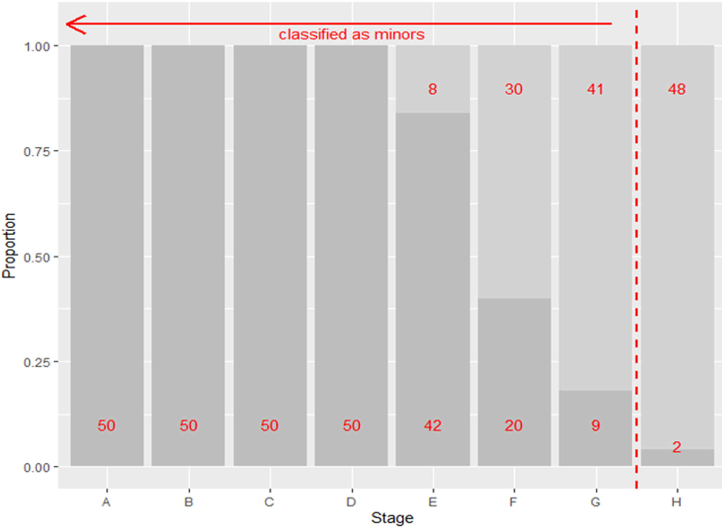
Age classification as a diagnostic testThe classification of individuals into one of two mutually exclusive binary states by comparison to a cut-off based on reference data describes a diagnostic test. In this example, individuals are classified into one of two age categories around a cut-off representing the legal age of majority (e.g. at 18 years), where the cases are considered to be minors. The contingency table of the simulated dataset in Table 2 shows the results from classifying individuals as either under 18 years (minors) or 18 years and above (adults) based on a cut-off between third molar stages G and H. This cut-off was chosen to minimise the number of minors misclassified as adults, and in the simulated data, only 2 out of a total of 273 individuals aged<18 years were misclassified as adults. The data was plotted to illustrate the proportion of adults and minors at each third molar stage and the placing of the age cut-off (Fig. 1).
The priority given to avoiding misclassifying minors as adults and therefore to correctly classifying them as minors, can be achieved by a test with a high sensitivity (a proportion of true positives amongst all cases). Applying this to the simulated data, the highest (i.e. 100%) sensitivity would only be achieved by accepting all individuals as minors irrespective of their third molar stage, since two minors in the simulated data had reached the highest stage, H. This would obviate the need for a test at all. However, sensitivity alone is not a sufficient criterion for evaluating whether a diagnostic test of sufficient accuracy can be developed from any given reference data for any given LIAT. Usually, a need for high sensitivity is balanced against the specificity for given cut-off, but for this, an acceptable rate of false positives or adults misclassified as minors, needs to be stipulated. This would be true for any prediction model based on multiple indicators or indicators measured on a continuous scale, as well as categorisation by comparison to a single ordinal indicator.
To motivate the approach to sample size calculation and to illustrate sampling artefacts described below, we applied a cut-off placed between stages G and H to our simulated data. The resulting diagnostic test has a sensitivity of 99%, a specificity of 38%, a positive predictive value (PPV) of 77% and a negative predictive value (NPV) of 96%.
Artefacts of samplingAge mimicryDetermining the suitability of a given indicator for estimating age depends on the distribution of age within the range of development for that indicator. However, estimating the distribution of age for an indicator can be biased by the distribution of age in a sample. It is axiomatic that the distribution of age in a random sample will converge to that of the population being sampled either with increasing sample sizes or through repeated sampling. This phenomenon was catalogued earlier in the related field of paleodemography.13 Dubbed “age mimicry” by Boldsen et al., the same authors have provided a framework on how to deal with this in predicting age based on their transition analysis of ordinal stages of skeletal traits.14 Gelbrich et al. highlighted this issue in the age estimation among the living, specifically applying this to Demirjian staging of third molar data.15 If a sample is taken randomly, then the distribution of third molar stages within each year of age should converge to that of the population with increasing sample size. Gelbrich et al. showed how the age distribution in, say, stage D third molar development follows the distribution of the sample and illustrated how the distribution of age within stage D, depends on the distribution of age in the sample – so-called age mimicry. Given the increasing sparsity of age categories above 17y, the mean age was stratified taking random samples within each year of age.15 Their solution to re-weight the sample to achieve a uniform distribution of ages is reasonable as a post hoc measure. However, the error in the less observed age categories can be inflated by the reweighting. Arguably, with prior knowledge of this issue, this should be pre-empted in the design of a study to collect reference data: Sampling could be stratified by year of age, with potentially sparser years of age oversampled to meet a pre-determined level of accuracy for those age groups.
Age range of reference sample and truncationIn the same study, Gelbrich et al. also highlighted the effect on the relationship between age and stage from truncation of the age range of the sample. Truncation of the age range for sampling could be considered a special and extreme case of age mimicry. In their 2010 paper, Gelbrich et al. illustrated this problem for describing the relationship between Demirjian stage and chronological age as a polynomial curve using Leipzig data. The last stage, which may include most of the population of adults, will be subject to truncation, which inevitably leads to a different parameterisation of the relationship between age and stage. Describing the relationship as a curve between age and stage may be done as part of the exploration of the data, or for providing an estimate of age from a prediction model.4,5 For providing an estimate of age, careful consideration needs to be given certain artefacts of regression and following the correct approach for calibration.16–18 However, while an estimate of chronological age is required, modelling the relationship between age and stage is not necessary to use a single ordinal (or binary) indicator for classifying individuals of unknown age as being either below or above a given cut-off.
Whether estimating age or classifying as minors and adults, researchers still need to consider the issue of truncation and specification of the age range when defining the sampling frame to create reference data. This is because the target population is likely to comprise individuals from only a limited range of ages around the age-cut-off. Those easily classified from other outwardly manifest characteristics (e.g. babies and older adults), will not likely be candidates for age evaluation and so would likely be excluded from the hypothesised reference population. However, the inclusion of the very young or the very old may introduce further problems for modelling age on stage with the inclusion of influential extreme values.
The simulated dataset covers a range of ages from 8 to 27y. Clearly, most individuals aged below 10y and aged nearly 30y are unlikely to be confused as an adult or minor respectively, and so these ages are unlikely to be among the target population. Therefore, truncation could realistically be applied to the simulated dataset, as if to make it conform to a hypothetical target population.
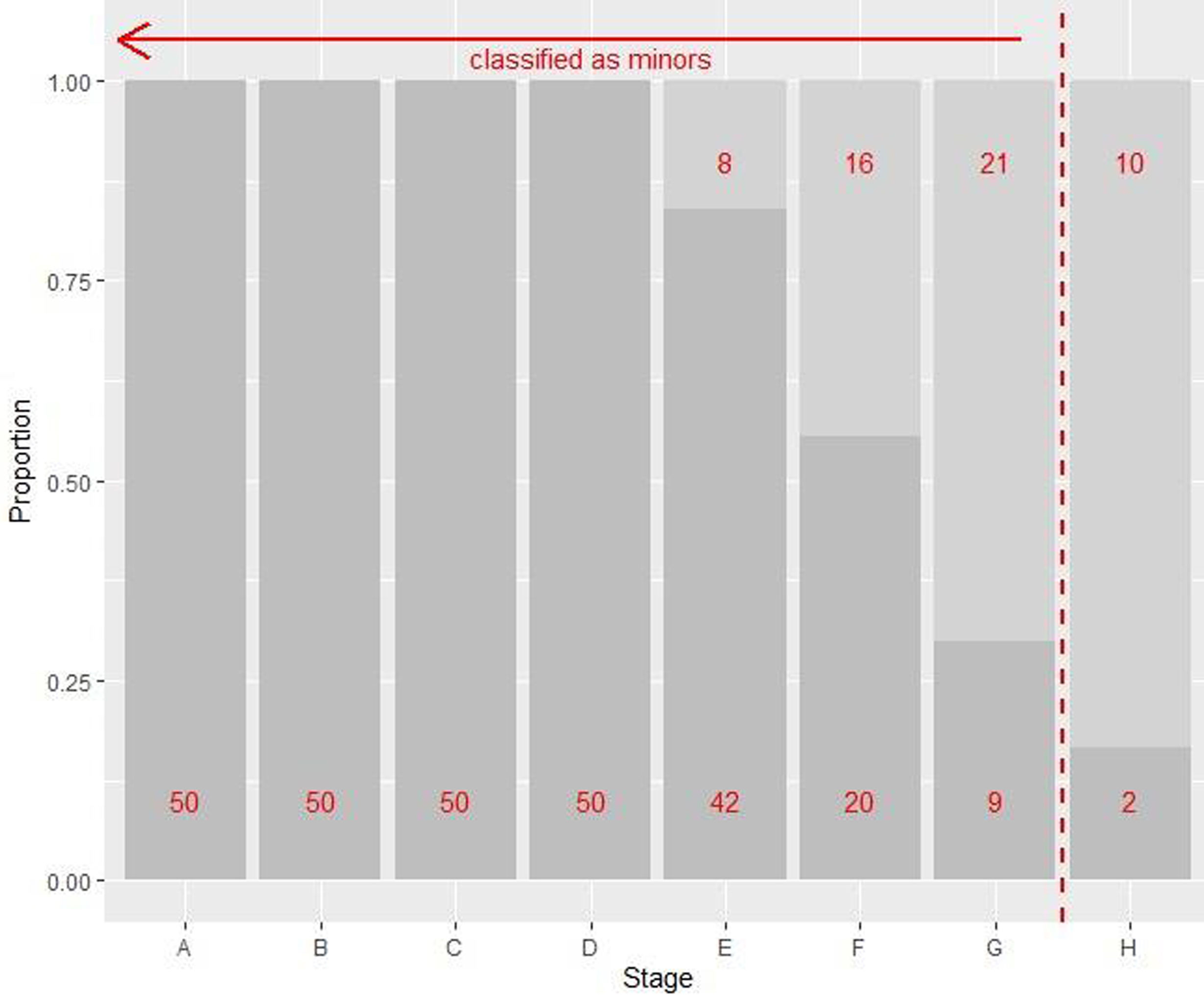
Truncating our simulated data to 21y reduces the number of individuals classified as adults by the legal threshold of 18y from 127 to 55, and both the specificity and negative predictive value are reduced from 38% to 18%, and 96% to 83%, respectively (Fig. 2). Truncation has also removed some adults with tooth stages below H, so PPV has increased from 77% to 86%. However, sensitivity remains the same at 99%. This is not unexpected, as sensitivity should remain the same, provided the cut-off for upper truncation does not fall below the cut-off of 18y.
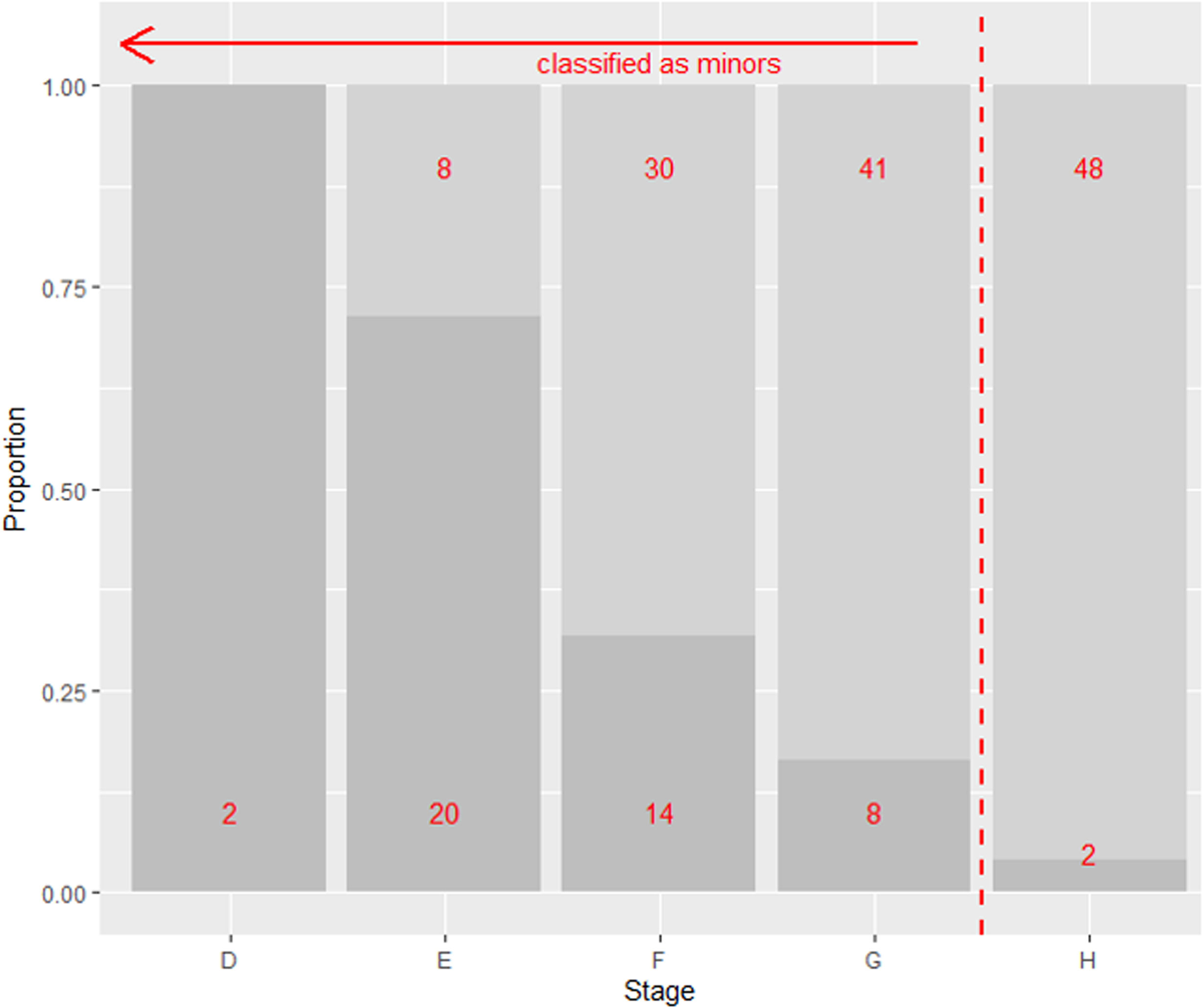
Reference data may also be truncated at the lower age range, by the exclusion of individuals, who are manifestly minors (e.g. infants). Truncating at 15y, removes over 90% of the minors from the simulated sample, yet the sensitivity of the test has only dropped from 99% to 96% (Fig. 3). This is consistent with what we should expect for cut-off (here between G and H) yielding a high sensitivity in these particular data. Generally, the number of true positives (correctly classified minors) needs to exceed the number of false negatives (minors incorrectly classified as adults) by a ratio of 19 to 1 to maintain a sensitivity of at least 95%. To maintain a sensitivity of 99% then this ratio should be 99 true positives to every 1 false negative. This rule also applies to the NPV, which remains at 96% after truncation at 15y. Specificity, which would be the proportion of adults correctly categorised as such, should be robust to changes at the lower end of the age range. Conversely, truncation of the lower age range should reduce the PPV, which has fallen from 77% to 36% with truncation at 15y, since this removes minors from the sample.
Designing reference data collectionFor estimating the age of unknown individuals, investigators require reference data on indicators of age-related development. Such data provide the basis for a model predicting age, which may then be used to classify individuals with respect to LIATs. However, classification may be done in parallel with age estimation if comparing directly to reference data on single indicators of age-related development.
Classification around the age cut-off can be framed as a diagnostic test, and thus the principles of diagnostic testing can be used to summarise the accuracy and precision of classification for a given set of reference data. Furthermore, this provides the basis for a sample size calculation, so that the reference data can support the classification of individuals to a desired level of accuracy around any given key age threshold.
Consideration given to sampling issues before collecting reference data is key to developing a successful model for estimating and classification around an age threshold. A sample size calculation will be an essential part of planning and may be based on a one-sided test of proportions for a desired level of sensitivity versus a minimum level of sensitivity.19 Understanding that investigators in age estimation typically prioritise a high sensitivity, we have provided an example table of sample sizes for a range of sensitivities compared to a range of minimum expected sensitivity values in Table 3, based on the exact, one-sided test of proportions in a single sample using the EnvStats package in R.20 While it is commonly understood that a high sensitivity is prioritised in age estimation involving minors, consensus is still required on an acceptable minimum level of sensitivity. Likewise, consensus is also needed over what second criterion should be applied in order to limit the number of false positives and how this should be measured (i.e. 1-specificity). This would provide better guidance on the required size of reference data, by combining the two criteria into a sample size calculation.21,22
Sample sizes, N, for number of individuals below a given LIAT for the exact tests of range of sensitivity values (H1, defined as H0 plus the given difference) against the null hypothesis (H0) of the minimum expect sensitivity at test powers of 80% and 90%.
| Minimum sensitivity (H0) | Power | Difference between test sensitivity (H1) and minimum sensitivity | |||
|---|---|---|---|---|---|
| 0.005 | 0.01 | 0.04 | 0.05 | ||
| 0.9 | 0.8 | 21,832 | 5354 | 286 | 179 |
| 0.9 | 0.9 | 30,180 | 7387 | 402 | 239 |
| 0.95 | 0.8 | 11,266 | 269 | 124 | – |
| 0.95 | 0.9 | 15,539 | 3701 | 153 | – |
| 0.99 | 0.8 | 1941 | – | – | – |
| 0.99 | 0.9 | 2546 | – | – | – |
Note: Sample sizes were incalculable for some combinations of minimum sensitivities and differences. For any given N number of individuals below the LIAT, the number of individuals above the LIAT must be collected according to the ratio that they exist in the population.
How reference data are collected is also important, given the sampling artefacts that may affect inference and prediction. If interest lies in describing the distribution of age within each stage of an ordinally measured indicator, then the issue of age mimicry may be pre-empted by stratifying sample collection by age group to achieve a uniform distribution of ages, or at least over-sampling sparse age categories in the reference population to meet a minimum level of precision in age prediction. However, for age classification around a given LIAT, the age distribution of the reference sample should be externally generalisable to its population. Therefore, while age mimicry may bias the estimation of age distribution of a given indicator, this may not be an issue per se for the classification of age around a LIAT, as long as the sample meets the desired property of being a representative sample of the population and the distribution of ages is accurately represented within each stage of indicator.
The age range of the reference sample will have ramifications for interpolation and predictive accuracy of age. Here, the age range of the reference sample will likely need to exceed that of the target population (individuals, whose age needs estimating) to reduce additional uncertainty at either end of the age range. However, in classifying age by direct comparison to age-related indicators and considering this as a diagnostic test, we demonstrated that the reference sample's age range may exert less influence on certain metrics of accuracy. Here, the need for a high sensitivity makes the misclassification of cases robust to truncation of the age range. However, consensus is still needed over what the second criterion should be for an acceptable rate of misclassification of non-cases.
Importantly, by framing age estimation as diagnostic test of age relative to any given legal age threshold, we have shown how the sensitivity (or specificity) from subsequent classification may be robust to the age range of the sample, provided:
- •
the sample is representative of the distribution of ages and indicator stages in the population,
- •
and that the given indicator (or age-related trait) can support classification around a LIAT with a high sensitivity (or specificity).
Direct classification around a LIAT relative to a given indicator obviates the need for an interim step of estimating age. It also provides an estimate of diagnostic accuracy and misclassification error without first having to estimate the prediction error from age estimation and potential bias arising from the model fitting issues in building the prediction model for age. Furthermore, in building an age prediction model, care has to be taken over the choice of age range as such a model may be sensitive to extreme values manifest in the lowest and highest stages of an indicator's stages. We have shown that direct classification according to a single indicator and potentially multiple indicators combined may be asymptotically more robust to the age range of a reference sample as classification around a chosen cut-off approaches 100% in the classification accuracy statistics. However, with the preference for a 100% sensitivity in classifying individuals as minors, a consensus is needed over the level of specificity or misclassification of adults as minors, as most data are unlikely to afford near perfect classification around both sides of a given cut-off.
ConclusionsPlanning in the collection of data for estimating age in legal medicine is key to avoiding problems arising from age mimicry and for ensuring the range of ages in the reference data reflect those of the test population. By considering age classification as a diagnostic test, we have shown how the priority for correctly classifying minors requires a test of age indicators that can offer high sensitivity. We have then shown how this can be robust to truncation of the sample by age. However, consensus is needed for a second criterion for classification accuracy, such as specificity, in addition to a high sensitivity to support proper planning and sample size calculations.
Ethical considerationsn/a.
FundingThe study was funded by the Deutsche Forschungsgemeinschaft (DFG, German Research Foundation) – Project No. 440395473.
Conflict of interestThe authors declare that they have no conflict of interest in relation to this article.
Funded by the Deutsche Forschungsgemeinschaft (DFG, German Research Foundation) – Project No. 440395473.


