

El propósito de este trabajo es representar las soluciones exactas de la ecuación de vorticidad barotrópica sobre la esfera unitaria S2 en rotación como una variedad, que son flujos zonales, ondas Rossby-Haurwitz y soluciones generalizadas llamadas modones. Se relacionan los métodos modernos de la teoría de funciones con la esfeoa definida como una variedad compacta y diferenciable. Cuando ésta se ha comprendido de forma correcta, se esclarece la noción abstracta de mapa local, cambio de mapa y atlas. Uno de los objetivos de este trabajo ns entender mejor lo solución de la ecuación de vorticidad barotrópica sobre la varieded S2 y su utilidad para identificar las propiedades de lac soluciones en la variedad Riemanniana (S2, g). Por lo tanto, estará disponible un tipo más general de espacio que también puede contener información geométrica y analítica sustancial sobre las soluciones a la ecuación de vorticidad barotrópica.
The purpose of this paper is to represent the exact solutions of the barotropic vorticity equations (BVE) on the rotating unit sphere S2 as a manifold, which are zonal flows, Rossby-Haurwitz waves and generalized solutions named modons. Modern methods of the function theory are connected to the sphere defined as a compact diferentiable manifold. When the differentiable manifold S2 is well understood, the abstract notion of local chart, change of chart, and atlases becomes evident. One of the aims of this paper is to better understand the solution of the barotropic vorticity equation on the manifold S2 and its usefulness to identify the properties of the solutions on the Riemannian manifold (S2, g). Therefore, a more general type of space will be available, which can also contain substantial geometric and analytic information about sotutions for the barotropic vorticity equation.
Let S2 ={x ∈ R3: | x |= 1} denote the unit sphere it R3. The large-scale dynamics of tire atmosphere on the rotating sphere S2 can approximately be governed by the non-linear barotropic vorticity equation (BVE), which can be written in the non-di-mensional from as:
where Ψ(λ,μ) denotes the stream function, μ=sinφ=cosθ,−π≤λ≤π,−π2≤φ≤π2,0<θ<π,λ the longitude, φ the latitude, and θ the colatitude. Δ is the Laplace-Beltrami operator on a sphere and J(Ψ, h) is the Jacobian.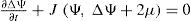
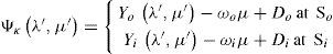
The following is a solution for Eq. (1) on the sphere proposed by Thompson (1982):

where (λ’, μ’) are the spherical coordinates relative to a rotated pole N’ with coordinates (λ0, μ0) with respect to the original system, and Yν is an eigenfunction of the operator Laplace-Beltrami with eigenvalue χνVerkley(1984) generalized Thompson's solution and demonstrated that Yν could be a set of eigenfunctions that contains more than only spherical harmonics. Then Eq. (2) describes a configuration in which the structure Yν moves through the zonal flow -ωμ with constant velocity cν and without changing size and shape. The pole of the primed system N’ that moves along a latitude at a constant angular velocity cν is given by
where χν is an eigenvalue for the spectral problem ΔYν= −χνYν. In particular, for spherical harmonics Y (λ’, μ’) of degree n corresponding to the eigenvalue χν = χn= n(n + 1), Eq.(2) is a Rossby-Haurwitz (RH) wave. RH waves have proven to be very useful to describe the large-scale wave structure of atmospheric circulation in middle latitudes (Rossby, 1939; Haurwitz, 1940). The solution modon is constructed to divide the sphere S2 into two regions (Tribbia, 1984; Verkley, 1984, 1987, 1990; Neven, 1992): an inner region Si centered around the pole N’, and an outer region So separated from the inner region by a boundary circle in which Ψ, q and its normal derivative Ψ’ are continuous. Modons are considered appropriate to describe some types of atmospheric blocking events (Verkley, 1990).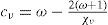
Hydrodynamic equations on manifolds were studied by Ebin and Marsden (1970), Szeptycki (1973a, b), Avez and Bamberger (1978), Ghidaglia et al. (1988), Temam (1987) and Ilyin (1993). The existence, unicity and regularity of the solution for the evolution equation (Eq. (1)) on S2 were proven by Szeptycki (1973a, b), Avez and Bamberger (1978), Ilyin (1993) and Skiba (2012). Ebin and Marsden (1970) dealt with the motion of an incompressible fluid on manifolds under a differential geometric point of view. Problems from the transition map between the charts are transferred to those of finding geodesics on the group of all volume-preserving diffeomorphisms, to which the methods of global analysis and infinite-dimensional geometry can be applied.
In this paper we study the manifolds S2 in terms of the stream function Ψ for an RH wave which is sufficiently smooth and for Wu-Verkley waves and modons which are weakly differentiable of higher orders. Section 2 deals with the compact differentiable manifold S2 and the way in which functions are constructed on this manifold. Section 3 shows the types of solutions that will be considered. Another aim of this paper is to deepen the understanding of the BVE solution on the manifold S2 and its usage for deriving the properties of solutions to the manifold (S2, g). The paper concludes with a summary in section 4.
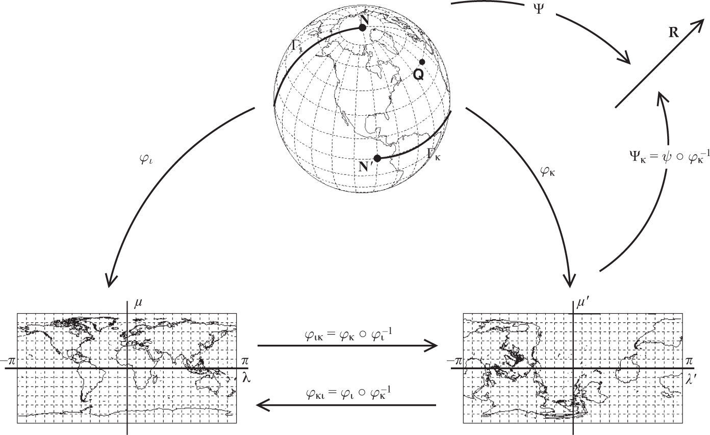
2Structure of functions on the manifold S2In this section we review some basic facts concerning to the manifold S2. We should recall that the unit sphere S2 is a compact and connected differentiable manifold. Indeed, because S2 is compact it is not possible to cover it with only one chart. A chart of S2 is then a pair (Ω,φ) where Ω is an open subset of S2, and φ is a homeomorphism of Ω onto some open subset of R2. Let us consider the two charts {(Ωι,φι), (Ωκ, φκ)} of class Cp for S2 where every chart corresponds to a geographical coordinate group. It is possible to define a coordinate chart that covers most of S2 by using the standard spherical coordinate map. Let φι denote the coordinate function, which maps from (x1, x2, x3) to angles (λ, θ) or to (λ, μ). The domain of φι−1 is the open set defined by λ ∈ (−π, π) and θ ∈ (0, π) (this excludes the poles). The inverse map φι−1 yields the parameterization x1 = cos λ sin θ, x2 = sin λ sin θ, x3 = cos θ and its variation φκ−1 yields the parameterization φκ−1 (λ’, θ’)=(cos λ’ sin θ’, cos θ’, sin λ’ sin θ’). The domain of φκ−1 in the open set defined by λ’ ∈ (–π, π) and θ’ ∈ (0, π). The charts Ωι,φι and Ωκ,φκ correspond to poles N and N’ on the sphere S2. N’ might be taken as the point (λ0=−π2φ0=0) in the old system and as the angle λ’ in this new north pole, so that the new international date line is the half circle Γκ={p∈S2:−π2<λ(p)<π2,θ=π2,} of the old equator in the x1x2- plane, on the front where x1 ≥ 0 (Richtmyer, 1981; Skiba, 1989; Pérez-García, 2001). The international date line, for the chart (Ωι, φι) is the half circle Γι={p∈S2:−π2<φ(p)<π2,λ=± π} in the x1x3 –plane. The chart covers (Ωι, φι) covers the sphere except for the set Γι, and the chart (Ωκ, φκ) similarly covers the sphere with the exception of a set Γκ. Hence the two charts {(Ωι, φι),(Ωκ, φκ)} together cover S2 and they constitute an atlas.
The local coordinates associated with the chart (Ωι, φι) are functions φι: Ωι,→R2, such that for p∈S2, φι(p)=(φι,1(p),φι,2(p))=(xι1(p), xι2(p))=(λ(p),μ(p))and φκ(p)=(xκ1(p),xκ2(p))=(λ'(p);μ'(p)) are local coordinates with respect to the chart (Ωκ, φκ) (Fig. 1).
, (Ωκ, φκ)} forms an atlas for S2: Ωι ∪ Ωκ = S2.")
To construct the map φℓ:S2→U⊂Rℓ2,ℓ=ι, κ a bijection with inverse φι−1:Uι→S2 defined as φι−1(xι1,xι2)=(1−(xι2)2cos xι1, 1−(xι2)2 sinxι1,xι2), and the φκ−1(xκ1,xκ2)=(1−(xκ2)2cos xκ1,xκ2,1−(xκ2)2sinxκ1), it is seen that every Uℓ is open. Hence each Ωℓ is an open subset of S2 and Ωι∪Ωκ cover S2.
Given two charts of the atlas {(Ωι, φι), (Ωκ, φκ)} with Ωκ ∩ Ωι≠ø, the transition maps φικ=φκ∘φι−1: Uικ→Uκι outline open sets of R2 into R2, where Uικ=φιΩι ∩ Ωκ and Uκι=φκΩκ ∩ Ωι. This determines a differentiable structure for S2, and φικ=φκ ∘ φι−1: is a diffeomorphism. It is then said that the atlas is of class Ck if the transition functions are of Ck.
Let x be any point of Uικ, and (φικ1(x),φικ2(x)) the coordinate of φικ (x); then φικi(x) is a continuous function on two variables. Now, if p ∈ Ωι ∩ Ωκ such that x = φι (p), and since φι(p) ∈ Uικ, we have the relations
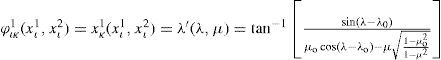

This is the transformation formula betwen the two local coordinate systems (xι1,xι2) and (xκ1,xκ2) defined on Ωκ ∩ Ωι. To obtain the relations between the unprimed and primed coordinate of any point Q on the sphere, Verkley (1984) examined the spherical triangle NQN’ and the application of the cosine rules to this triangle, deriving explicit expressions for the transformation between the two coordinate systems as given by (4) and (5).
Let Ωι ∩ Ωκ≠ø and set J φικ as the Jacobian matrix of map φικ, so we can verify that
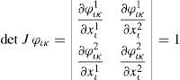
Then det J φικ > 0. Hence, it is said that if manifold S2 is oriented for every pair Ωι, Ωκ of intersecting local coordinate neighbourhoods, det J φικ > 0.
Indeed we can regard the coordinate as a device to decide which of many functions ψ on S2 are to be differentiable. Since Ωι is just a set, it makes no sense to ask that ψ: Ωι→ R be differentiable (Matsushima, 1972; Loomis and Sterberg, 1990). However, we can consider the map Ψι=ψ ∘ φι−1:φι (Ωι)→R Then ψ ∘ φι−1 is a function defined on an open φι(Ωι)⊂R2, and we know what it means for such a function to be differentiable or smooth (see Fig. 1). Consider now what happens when we change coordinates to some other chart, lets say (Ωκ, φκ) for convenience, assuming that Ωι = Ωκ, Then it is possible for ψ ∘ φι−1 to be differentiable but ψ ∘ φκ−1 is not. To compare both, let ψ ∘ φι−1=ψ ∘φκ−1 ∘ (φκ ∘ φι−1) where the map φκ∘φι−1:φι(Ωι)→φκ(Ωκ) is a bijection between open subsets of R2. Then a sufficient condition for ψ ∘ φι−1 to be differentiable if φ ∘ φι−1 is, is that ’φκ ∘ φι−1 is also differentiable. We often write Ψ for the composite function ψ ∘ φι−1
Lets take a curve τ : (−1, 1) → S2 with τ (0) = p. In a local chart τ is given by xιi=τi(t). On the manifold S2, one can define a vector U tangent to the parametrized curve τ at any point p on the curve. The tangent vector U is given by a column vector u whose components uιi are dτidt0, (i = 1, 2), with the initial condition τ (0) = p. If we use another coordinate system corresponding to the chart (Ωκ, φκ) by xκi then the tangent vector U is given by a column vector v with components υκi. According to the chain rule, the column vectors u and v are related by υκi=uιj∂xκi∂xιj. The expression uιi∂∂xιj is the partial differential operator in the direction of the tangent vector.
The space TpS2 is called the tangent space of S2at p, and TpS2 is a two-dimensional vector space. For each u ∈ TpS2 we shall write u=uιi∂∂xιj=u1∂∂λ+u2∂∂θ, where uιi are the contravariant components of u. It is well known that on the manifold S2 an inner product is defined at each tangent space TpS2. Now lets present a basis in which we denote the coordinate system corresponding to the chart (Ωι, φι) by {xιi}=(λ,μ), and for any ψ: S2 → R define the vectors (∂∂xιj)p by (∂∂xιj)pψ=(∂ψ∘φι−1∂xιi)φι(p), so that they are independent since (∂∂xιj)pxιj=δij Let (nˆ=(1−(xι2)2cosxι1,1−(xι2)2sinxι1,xι2) be the outward normal to S2 in R3; without any loss of generality we may assume that the vectors eλ=∂nˆι∂xι1, eμ=∂nˆι∂xι2 form a basis for TpS2.
We will denote the vector space of a vector field on S2 by Γ(S2) A tangent vector field on S2 is a smooth map u: S2 → T S2 such that, for any x ∈ S2, u(x) ∈ TxS2. At the chart (Ωι, φι), for x ∈ Ωι, the vector functions u ∈ TxS2 and v ∈ Γ(S2) have components u=up1eλ+up2eμ and v=υp1eλ+υp2eμ, respectively, being these up upi=upxιi=uλ,uμ the components of up as the vectors of the unitary base indicated by eλ, and eμ in the directions λ and μ, respectively.
Let us recall that an oriented Riemannian manifold is a pair (S2, g) where S2 is the oriented compact manifold and g a Riemannian metric on S2, which assigns a length vgp∈R+. The g on S2 is a smooth (2, 0)-tensor field on S2 such that for any p ∈ S2, gp: Tp(S2) × Tp(S2) → R is a scalar product on the tangent space Tp(S2), and in any chart (Ωι, φι) of S2, its components
form a symmetric matrix, with its inverse denoted by (gij) = (gij)-1, and g = det(gij) = 1 – μ2. The length of a tangent vector v ∈ TpS2 is defined as usual, v=gpv,v12=v·v12 Moreover, the inner product on T S2 is given by u . v = gijuiνj for u, v ∈ TS2.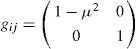
Let (S2, g) be the smooth Riemannian manifolds of S2. Let us now recall some operators arising in partial differential equations on the sphere as manifold. Given the scalar function ψ : S2 → R, the gradient of ψ, is given by the vector field grad ψ: S2 → TpS2, for which
where eˆλ =11−μ2eλ and eˆμ=1−μ2 eμ.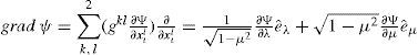
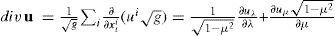
If u ∈ Г(S2), the divergence of u is the function on S2 which on the chart (Ωι, φι) is given by
A linear connection D on S2 is a map D: T(S2) × Г(S2) → T(S2) called the covariant derivative and the usual notation for D(U, V) is DUV. Let (Ωι, φι) be a chart and as one can observe, the vectors (eλ=∂∂λ,eμ=∂∂μ) can be nonconstant. An easy notation is set ∇i=D∂∂xi (eg. Hebey, 2000). There are smooth functions Γijk:Ωι→R such that for any i, j, and any p ∈Ωι,
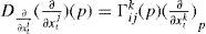
where Γijk are the Christoffel symbols, defined by Γijk=12∑l=12gkl(∂glj∂xιi+∂gil∂xιj+∂gij∂xιl).On the chart (Ωι, φι), we have Γ111=0,Γ112=−2μ1−μ2,Γ121=cot θ=μ1−μ2,Γ122=0,Γ221=0 and Γ222=0
The fundamental operator which we study is the Laplacian Δ, then for real or complex valued functions, Δ is the Laplace-Beltrami operator on S2 and it is given by

This operator satisfies some properties: Δg, is selfadjoint, symmetric and non-negative (Aubin, 1998). Thus, the operators div, grad and Δg on the manifold S2 have the conventional meaning.
Let (S2, g) be a compact oriented Riemannian manifold, with metric g. The metric and the orientation are combined to give a volume element dυg on S2, which can be used to integrate functions on (S2, g). In order to apply the integral calculus on the oriented manifold S2, we define a volume element to be a two-form ω = dυ which is defined on all of S2. For every chart (Ωℓ, φℓ) which is consistently oriented with S2, the coordinate expresion for ω=dυl is Φldxl1Λdxl2 where Φℓ is a partition of unity subordinate to the covering Ωl, l=ι,κ
On the Riemannian manifold (S2, g), at the chart (Ωι, φι); a volume form η = dυg defines a Lebesgue measure on S2 by dυg=η=gdxl1 Λdxl2 Then
wheredxl=dxl1dxl2 defines a Lebesgue measure on R2.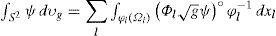
Let C∞(S2) denote the set of infinitely differentiable functions of compact support ψ(x). At μ = ± 1 the functions are smooth, together with the periodic boundary condition at λ with period 2π. If we define the usual Hilbert space L2(S2) to be the completion of C∞(S2) with respect to the inner product
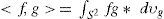
and norm f={∫s2f2dυg}12, g* is the complex conjugate of function g. Let (S2, g) be the compact Riemannian manifold and dυg the Riemannian volume element. Then functional spaces (Sobolev and the Holder spaces) can be defined on S2 as well (Skiba, 2012). For each p ∈ R with 1≤ p < ∞ we associate a Banach space

with respect to the norm
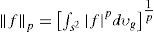
and ess sup | f | < ∞ if p = ∞. L2(TS2) represent the Hilbert space of the vector fields U : S2 → TS2 endowed with the inner product in L2(S2) induced by g in Tp(S2) (see Díaz and Tello, 1999; Hebey, 2000).
We now turn to the eigenvalue problems for Δg: We usually seek to find all eigenvalues γ for which there is an eigenfunction Y such that ΔgY = –γY. Then, which information about geometry of (S2, g) is encoded by the eigenvalues?. The structure of eigenfunctions: Lp norms and relations to RH waves or modons.
Global harmonic analysis is the study of the spectral theory of the Laplacian Δg on a compact Riemannian manifold (S2, g), and its relation to the global geometric structure. Since (S2, g) is compact, there exists an orthonormal basis {Yj} of smooth eigenfunctions and the spectrum of Δg is a discrete set {γ0 = 0 < γ1 ≤ γ2 ≤ γ3 ≤ ...}. Recent developments show that the non-zero eigenvalues also contain substantial geometric and analytic information. The solution modon constructed by Tribbia (1984), Verkley (1984, 1987, 1990) and Neven (1993) proposed the use of eigenfunctions {Yj} as basic geometric structures.
The space of spherical harmonics of degree n on S2, which coincides with the eigenspace of operator – Δg corresponding to the eigenvalue γn =χn=n(n+1), is denoted by Hn. Self-adjoint operators have the property that its eigenfunctions with different eigenvalues are orthogonal, which implies that the eigenspaces Hn are orthogonal and have 2n+1 dimensions. On the sphere, the homogeneous harmonic polynomials span the set of all polynomials, which in turn are dense in L2. Our spherical harmonics therefore span L2. If we take a basis within each eigenspace then this collection will give a basis for L2 of the sphere. The harmonics spherical term was introduced by Kelvin on potentials studies (Hobson, 1931) and is understood as the development of a function in terms of this series of spherical harmonics.
The spaces Hn and Hk (n ≠ k) are mutually orthogonal in L2(S2). Then there is the orthogonal projection Yn : L2(S2) → Hn, and so smooth functions Ψ ∈ L2(S2) on the sphere S2 have a development in spherical harmonics,
where Ynλ,μ=∑m= −nnΨnm Ynmλ,μ is the homogeneous spherical polynomial of degree n from Hn, and Ψnm= < Ψ,Ynm> is the Fourier coefficient of Ψ. The 2n + 1 spherical harmonicsof degree n and zonal number m (–n ≤ m ≤ n) form an orthonormal basis in Hn. Here the numbers Cnm are the normalizers in L2(S2), given byCnm=2n+14πn−m!n+m!12 and Pnm are the associated Legendre functions given by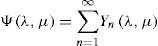

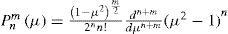
Considering that an oriented compact Riemannian manifold is a pair (S2, g) where S2 is the oriented compact manifold and g a Riemannian metric on S2, we can define in it covariant derivatives and various notions of curvature. When a manifold also has a group structure (so that multiplication and inversion are smooth), a very interesting structure called a Lie group (Bihlo, 2007; Bihlo and Popoych, 2012) arises. Even if a manifold S2 is not a Lie group, there may be an action : G × S2 → S2 of a Lie group G on S2, and under certain conditions S2 can be viewed as a “quotient” G/K, where K is a subgroup of G (Richtmyer, 1981). When S2 ≅ G/K as above, certain notions on G can be transported to S2, then we say that S2 is a homogeneous space. As an example of the last point we could mention the theory of spherical harmonic expansion on the S2, which is a homogeneous space for the rotation group O(n+1). The surface spherical harmonics are eigenfunctions for the Laplace-Beltrami operator, which is a rotation invariant (Helgason, 1984). Harmonic analysis is concerned with the representation of functions as the superposition of basic waves, the study and generalization of the notions of Fourier series as well as the Fourier transforms.
Elements of harmonic analysis on the sphere can be found at Stein and Weiss (1971). After introducing the manifold S2 and the Riemannian manifolds (S2, g), a general type of spaces (Besov and Triebel-Lizorkin spaces) on the sphere may also be introduced (Narcowich et al., 2006). Using the power of a Laplace operator, the Sobolev space on Riemannian manifolds can also be incorporated as a field currently undergoing great development (Aubin, 1998; Hebey, 2000).
3Exact solutions to the barotropic vorticity equation on the manifold S2Let {(Ωι, φι)},ℓ=ι, κ be an atlas of S2 and ψ: S2 → R the streamfunction of class Cr. We can consider that the map Ψ=ψ∘φι−1:φιΩι→R and ψ∘φι−1 is the streamfunction defined on an open Uι = φι (Ωι) ⊂ R2 and that it is of class Cr.
To simulate the time evolution of a two-dimensional nondivergent and inviscid flow for a rotating sphere, S2 is governed by a non-linear barotropic vorticity equation, which can be written in the non-dimensional form as

where Jc,q=∂c∂λ∂q∂μ−∂c∂μ∂q∂λ=k×∇c·∇q=u·∇q is the jacobian, u = k×∇c=uλ,uμ=−1−μ2∂c∂μ,11−μ2∂c∂λ is a tangent velocity vector, gradc=∇c=11−μ2∂c∂λ,1−μ2∂c∂μ,c=Ψ,ξ=ΔΨ=div grandΨ, is the relative vorticity q =ΔΨ + 2 μ is the absolute vorticity and k is a unit outward normal vector. The velocity vector field u having the components (uλ,uμ) is solenoidal: ∇ · u = 0 Throughout decades the nonlinear barotropic vorticity equation has been successfully used to describe low frequencies and large-scale barotropic processes of atmospheric dynamics. Despite the simplicity to this nonlinear equation, it contains the principal elements that describe the complexity of atmospheric behavior (Simmons et al., 1983; Skiba, 1997). The four types of exact solutions to Eq. (1) known up to now are described below:
- •
The zonal flows and Rossby-Haurwitz (RH) waves (Haurwitz, 1949), called classical solutions, differentiated from the generalized solutions which are not so smooth.
- •
The first generalized solutions of Eq. (6), kown as modons, were originally constructed by Tribbia (1984) and Verkley (1984, 1987, 1990) by using two eigenfunctions for the Laplace operator of different degrees.
- •
Later on, Neven (1992) gave generalized solutions in the form of a quadrupole modon.
- •
Wu and Verkley (1993) constructed generalized global solutions composed of two RH waves (Pérez-Garcia and Skiba, 1999).
In the present work, zonal flows, homogeneous spherical polynomials flows, RH waves, and modons on the manifold S2 are considered.
3.1Classical solutionsLet us consider the zonal flows, homogeneous spherical polynomials flows and Rossby-Haurwitz (RH) waves.
Proposition (zonal flow). Let {(Ωι, φι)}, ℓ = ι, κ be an atlas of S2 and the streamfunction ψ : S2 → R of class Cr. Then the zonal flow map Ψι=ψ∘φι−1:Uι⊂Rι2→R of Cr defined as
is an exact solution of the vorticity Eq. (6) for any bn.
Proof. The demonstration, obtained from Eq. (6), is quite trivial.
Proposition (homogeneous polynomials).
Let {(Ωι, φι)},ℓ = ι, κ be an atlas of S2 and the streamfunction ψ : S2 → R of class Cr. Then the homogeneous spherical polynomial map Ψι=ψ∘φι−1:Uι⊂Rι2→R of degree n ≥ 2 defined as
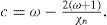
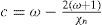
is an exact solution to the vorticity Eq. (6), where am can be a complex factor and

is the angular phase speed.
Proof. Given Ψι ∈ Hn, we define Ψιλ, μ, t= Ψn(λ−ct, μ)=∑m=−nnamYnmλ−ct, μ, then ∂Ψn∂t=−2Ψ′, and ∂Ψn∂λ=Ψ′, where Ψ′=∑m=−nnimamYnm(λ−ct, μ). If, in addition, we have the following expression
we have from BVE (Eq. (6)). It follows that c =−2χn.

Proposition (Rossby-Haurwitz waves). Let {(Ωι, φι)}, ℓ = ι, κ be an atlas of S2 and the streamfunction ψ : S2 → R of class C∞.Then, the map Ψι=ψ∘φι−1:Uι⊂Rι2→R of C∞ define as
with n ≥ 1 is called Rossby-Haurwitz (RH) waves.

It is an exact solution of the vorticity Eq. (6) if the angular phase speed of the RH wave
Here ω is the super-rotation velocity and each Hn corresponds to the eigenvalue χn = n(n+1).
Proof. Here Ψι is expressed by
where Ψnλ−ct, μ=∑m=−nnamYλ−ct, μ. We can notice thatwhich implies that


Furthermore:
where Ψ′=∑m=−nnimamYnm(λ−ct, μ); so that from BVE (Eq. (6))

Hence
so thatand thus the proposition is proved.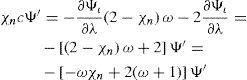
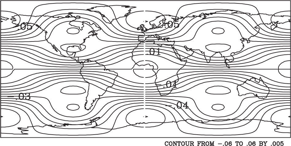
The streamfunction of the stationary RH(2,5) wave
with the parameters defined by (m, n) = (2, 5), a = .007 and ω=23(χ3−2) is given in Figure 2.
.")
Pérez and Skiba (2001) and Skiba and Pérez (2006) developed a numerical spectral method for the normal mode instability study of the arbitrary steady flow of an ideal nondivergent fluid on a rotating sphere, and Skiba and Pérez (2006) tested this method for the RH(2,5) wave. Pérez-García (2014) constructed a basic flow regarded as a sum of a zonally symmetric flow (Eq. 7 and a Rossby-Haurwitz wave component (Eq. 9.
3.2Generalized solutionsDenote the spherical distance between two points of S2 by d(.,.). Let N’ be the north pole of the chart coordinate (Ωι, φκ). Then a disk or inner region Si on the sphere is defined as Si=DN′,φa={s ∈ S2| dN′,s<φa}, such that 0<φa≤π2 The solution modon is constructed (Tribbia, 1984; Verkley, 1984, 1987, 1990; Neven, 1993) to divide the sphere S2 into two regions: an inner region Si centered around the pole N’, and an outer region So separated from the inner region by a boundary circle ∂DN′,φa={s ∈ S2| dN′,s<φa}, on which ψ, q and ψ’ are continuous.
For Si a solution of the Eq. (2) form is chosen with an eigenfunction Y (λ’, μ’) which has its singularity in the outer region. The same type of solution is chosen for the outer region, but such that Y (λ’, μ’) has its singularity in the inner region. Then both solutions are combined as smoothly as possible on the boundary circle ∂DN′,φa (Tribbia, 1984; Verkley, 1984, 1987).
To construct the Verkley (1984) modon or the Neven (1992) cuadrupole modon on the manifold S2, it is interpreted as:
Proposition. Let {(Ωℓφℓ)}, ℓ = ι,κ, be an atlas of S2, and ψ = ψ1 + ψ2 : S2 → R the streamfunction of Cr. Then

Proof. Let ψ1 and ψ2 be two real-value functions of class Cr defined on the differential manifolds S2. We define their sum by setting Ψι=(ψ1+ψ2)∘φι−1=ψ1∘φι−1+ψ2∘φι−1 for any chart (Ωι,φι) Since the sum of two functions of class Cr on S2 are functions of class Cr, the proof of this formula can be obtained by the expression
where φικ(λ, μ)=(φικ1 (λ, μ), φικ2 (λ, μ))=(λ′(λ, μ),μ′(λ, μ))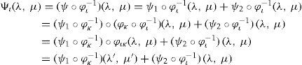
Decompose now the streamfunctions into an eigenfunction part (ψ1∘φκ−1) (λ′, μ′)=Yν(λ′, μ′) and a zonal part (ψ2∘φι−1) (λ, μ)=−ωμ+D where –ωμ is a solid-body rotation and D a constant. In chart (Ωκ, φκ) with coordinates (λ’, μ’), the north pole N’ moves along a circle of constant latitude with constant angular velocity cν. In the primed coordinates, Verkley (1984, 1987) modons have the form
which consists of a dipole and a monopole component:
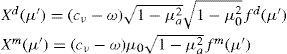
where μ0 = sen φ0μa = sen φa. The functions fd(μ) and fm(μ) are defined as
and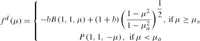
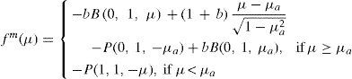
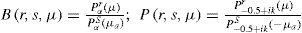
where b=k2+14+2α(α+1)−2 and
The fact that
is a solution to Eq. (6) is due to the work of Verkley (1984), which I will not reproduce in this paper. Yν is an eigenfunction of the Laplace-Beltrami operator and χν = –ν(ν + 1) is the eigenvalue of Yν. The Legendre functions Hμ=Pνmμ and Hμ=Qνmμ are solutions to the Legendre differential equation of hypergeometric type, where Pνm(μ) is a Legendre function of the first kind and Qνm(μ) is a Legendre function of the second kind for order m such that ν is the complex degree. The explicit expresion for Pνmμ and Qνmμ with –1 < μ < 1 can be found in Abramowitz and Stegun (1965) or Verkley (1984).
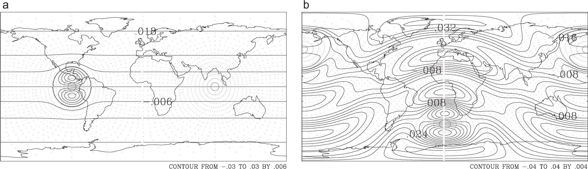
By using a grid of 5 × 5° upon the local coordinate associated with the chart (Ωκ,φκ), the Verkley, 1984 modon was numerically generated. Using Eqs. (4) and (5) a workable Gaussian mesh of (128, 64) points upon the geographical coordinate group (Ωι, φι) was also generated. This mesh was mapped onto the local coordinates system associated to the chart (Ωκ,φκ). The values of Ψκ were interpolated on the Gaussians points (128, 64) by implementing a nine- point Lagrange interpolation scheme. The resulting function, i.e. the Verkley, 1984 equatorial modon viewed on the geographical coordinate group (Ωι, φι), is shown in Figure 3a. This small modon was defined by the following parameters:

 with (a) k = 10., a = 10.,φa= 66.14°, λ0 = 270.0° and φ0 = 0.°; the uniform Verkley modon (1990) at (b) σ = 8.06, φa = φa=5π12,λ0=180.0°, φ0 = 180.0° and φ0 = 45.0°. The curve points are the spherical coordinates relative to a rotated pole N’(270.0°, 0.°) at (a) N’(180.0°, 45.°) at (b) with respect to the original system.")
Streamfunction isolines of equatorial Verkley modon (1984) with (a) k = 10., a = 10.,φa= 66.14°, λ0 = 270.0° and φ0 = 0.°; the uniform Verkley modon (1990) at (b) σ = 8.06, φa = φa=5π12,λ0=180.0°, φ0 = 180.0° and φ0 = 45.0°. The curve points are the spherical coordinates relative to a rotated pole N’(270.0°, 0.°) at (a) N’(180.0°, 45.°) at (b) with respect to the original system.
A numerical spectral model was used to simulate this small-size modon in Pérez-García and Skiba (1999), and in Skiba and Pérez-García (2009) a numerical spectral method for normal mode stability study of ideal flows on a rotating sphere was tested for this isolated steady modon constructed by Verkley (1984).
Studies done by Illari (1984) and Crum and Stevens (1988) noted that the values of isentropic potential vorticity are relatively low and uniform in the blocking region. In our following argument we consider that Verkley's modon (1990) provides a better and more uniform description of atmospheric blocking. Our interest lays within the fields that build this phenomenon. These solutions are characterized by a region Si in which q is constant, and an outer region So separated from the inner region by the boundary circle ∂D, on which Ψ and q are both constant, i.e., Ψ = d and q = b.
In the primed coordinates the Verkley (1990) modon has the form
where solid-body rotation terms can be expressed in primed coordinates using Eqs. (4-5), such that in chart (Ωι, φι) the eigenfuctions at the outer region and inner region are Δ′Yo=−χoYo; Δ′Yi=ei being χo and ei constants. Certain requirements of continuity must be met to generate these functions over the circle ∂D. We require continuity in and the first and second derivative in φ’ at φa.
To construct the Verkley, 1990 uniform modon on the manifold S2, it is interpreted as:
Proposition. Consider an atlas {(Ωℓ, φℓ)}, ℓ = ι,κ, of S2 and let ψ = ψ1 + ψ2 : S2 → R be the stream-function of Cr. Then

Proof. Let ψ1 and ψ2 be two real-value functions of class Cr defined on the differential manifolds S2. We define their sum by setting Ψκψ1+ψ2∘φκ−1=ψ1∘φκ−1+ψ2∘φκ−1 for any chart (Ωκ, φκ). Since the sum of two functions of class Cr on S2 are functions of class Cr, the proof of the proposition follows from:
because λ,μ=φκιλ′,μ′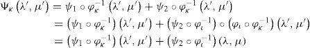
According to Verkley (1990), to express the modon in a more explicit manner, the functional forms Yo and Yi of the eigenfuntions are:
where As and Bs are constant. The special functions Sσmθ′=Pσm−cos θ′ and Tm(θ’) were given by Verkley (1990).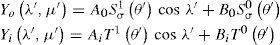
We have also reproduced numerically the uniform modon constructed by Verkley (1990) using the parameters φa=5π12, σ=8.06; ωo=0.028, and when the modon center is in the point λo=180°,φo=π4 (Fig 3b).
4ConclusionsThe exact solutions of the barotropic vorticity equation on the rotating unit sphere as a compact differentiable manifold without boundary, which are zonal flows, homogeneous spherical polynomial flows, Rossby-Haurwitz waves and generalized solutions named modons, were represented in this paper. A concrete notion of local chart, change of charts, and atlas for the manifolds S2 was developed. An atlas {(Ωι, φι), (Ωκ, φκ)} was constructed for S2, where every chart corresponds to a geographical coordinate group that covers most of S2. The transition maps φικ=φκ∘φι−1:φιΩι∩Ωκ→φκΩι∩Ωκ and φκι=φι∘φκ−1:φκΩκ∩Ωι→φιΩκ∩Ωι were also constructed, and the exact solutions of the barotropic vorticity equation in a manifold context were studied. This work also formulates on the manifolds S2 in terms of the stream function ψ: S2 → R, for RH waves which are sufficiently smooth, and for Wu-Verkley waves and modons which are differentiably weak. RH waves as solutions ψ∘φι−1 of the barotropic vorticity equation on the manifolds S2 are presented at the local coordinate associated with a chart (Ωι, φι). The way in which the modon solution ψ∘φκ−1 can be constructed in the chart (Ωκ, φκ), where ψ is C2, is investigated too. In the chart coordinate (Ωκ, φκ), the Verkley (1984, 1987) modons have the form
To construct the Verkley (1990) uniform modon on the manifold S2, it is interpreted as

when the modon center is in the point λo = 270; φo = 0. However, to contruct the verkley (1984,1987, 1990) with N’ a point arbitrary on the sphere S2 a collection of pairs (Ωι, φι) (i > 2) is needed. Our viewpoint here was to understand the solution of the barotropic vorticity equation on the manifold S2 and its use to derive properties of the solutions to the Riemannian manifold (S2, g).
The author is grateful to A. Aguilar in the preparation of the figures. N. Aguilar, A. Alazraki, and C. Amescua gave valuable suggestions for improving the manuscript.