

Se considera la ecuación no lineal de vorticidad barotrópica (BVE) que describe la dinámica de vórtice de un fluido incompresible, viscoso y forzado sobre una esfera giratoria. Se estudia el comportamiento asintótico de las soluciones de la BVE no estacionaria cuando t → ∞. Se dan las formas particulares de la fuente externa de vorticidad que garantizan la existencia de un conjunto atractivo acotado en el espacio de fase de las soluciones. Se muestra que el comportamiento asintótico de las soluciones BVE depende de la estructura y la suavidad del forzamiento externo. También se dan tres tipos de condiciones suficientes para la estabilidad asintótica global de soluciones BVE, suaves y débiles. Se consideran conjuntos atractivos simples de un fluido viscoso incompresible en una esfera cuando el forzamiento es un polinomio cuasi-periódico en tiempo. Cada conjunto atractivo representa una solución cuasi-periódica de la BVE del subespacio complejo Hn de dimensión (2n + 1) que contiene los polinomios esféricos homogéneos de grado n. Su trayectoria es una espiral abierta densamente enrollada alrededor de un toro 2n-dimensional en Hn, y por lo tanto su dimensión de Hausdorff es igual a 2n. Cuando el número generalizado de Grashof G se vuelve suficientemente pequeño, el dominio de atracción de tal solución espiral se expande de Hn a todo el espacio de fase de la BVE. Se muestra que para un valor determinado G, existe un número entero nG tal que cada solución espiral generada por un forzamiento de Hn con n ≥ nG es estable global y asintóticamente. Así, demostramos la diferencia en el comportamiento asintótico en los casos en que el número de Grashof G está fijo y acotado, pero el forzamiento es estacionario o no estacionario. En el caso del forzamiento estacionario, la dimensión del atractor de fluido está limitada desde arriba con el número G. Y en el caso del forzamiento no estacionario, la dimensión de la solución atractiva espiral (igual a 2n) puede ser arbitrariamente grande si el grado n del forzamiento polinomial cuasi-periódico crece. Dado que las funciones cuasi-periódicas de pequeña escala, a diferencia de las funciones estacionarias, representan más adecuadamente el forzamiento en la atmósfera barotrópica, este resultado es de interés meteorológico y muestra que la dimensión de los conjuntos atractivos no sólo depende de la amplitud del forzamiento, sino también de su estructura espacial y temporal. Este ejemplo también muestra que la búsqueda de un atractor global de dimensión finita en la atmósfera barotrópica no está bien justificada.
The nonlinear barotropic vorticity equation (BVE) describing the vortex dynamics of viscous incompressible and forced fluid on a rotating sphere is considered. The asymptotic behavior of solutions of nonstationary BVE as t → ∞ is studied. Particular forms of the external vorticity source are given that guarantee the existence of a bounded attractive set in the phase space of solutions. The asymptotic behavior of the BVE solutions is shown to depend on both the structure and the smoothness of external forcing. Three types of sufficient conditions for global asymptotic stability of smooth and weak BVE solutions are also given. Simple attractive sets of a viscous incompressible fluid on a sphere under quasi-periodic polynomial forcing are considered. Each attractive set represents a BVE quasi-periodic solution of the complex (2n + 1)-dimensional subspace Hn of homogeneous spherical polynomials of degree n. The Hausdorff dimension of its trajectory, being an open spiral densely wound around a 2n-dimensional torus in Hn, equals to 2n. As the generalized Grashof number G becomes small enough then the domain of attraction of such spiral solution is expanded from Hn to the entire BVE phase space. It is shown that for a given G, there exists an integer nG such that each spiral solution generated by a forcing of Hn with n ≥ nG is globally asymptotically stable. Thus we demonstrate the difference in the asymptotic behavior of solutions in the cases, then Grashof number G is fixed and bounded, but the forcing is stationary or non-stationary. Whereas the dimension of the fluid attractor under a stationary forcing is limited above by G, the dimension of the spiral attractive solution (equal to 2n) may become arbitrarily large as the degree n of the quasi-periodic polynomial forcing grows. Since the small-scale quasi-periodic functions, unlike the stationary ones, more adequately depict the forcing in the barotropic atmosphere, this result is of meteorological interest and shows that the dimension of attractive sets depends not only on the forcing amplitude, but also on its spatial and temporal structure. This example also shows that the search of a finite-dimensional global attractor in the barotropic atmosphere is not well justified.
The nonlinear barotropic vorticity equation (BVE) describing the vortex dynamics of a viscous incompressible and forced fluid on a rotating sphere is considered, which takes into account the Rayleigh friction, the sphere rotation, the external vorticity source (forcing) F(t, x), and the turbulent viscosity term of common form ν(−Δ)s+1ψ, where s ≥ 1 is an arbitrary real number. The case s = 1 corresponds to the classical form used in Navier-Stokes equations (Ladyzhenskaya, 1969; Szeptycki, 1973a, b; Temam, 1984; Tribbia, 1984; Ilyin and Filatov, 1988), while the case s = 2 was considered for example in Simmons et al. (1983), Dymnikov and Skiba (1987a, b), and Skiba (1989). The turbulent term of such form for natural numbers 5 is applied in Lions (1969) for studying the solvability of Navier-Stokes equations in a limited area by the artificial viscosity method. The unique solvability of nonstationary BVE for arbitrary real number s ≥ 1, as well as the existence of weak solution to the stationary BVE, was shown in Skiba (2012). A condition guaranteeing the uniqueness of such steady solution is given in the same work.
Many works have been devoted to the study of large-time behavior of 2D vorticity equation solutions (Temam, 1985; Marchioro, 1986; Ladyzhenskaya, 1987; Constantin et al., 1988; Giga and Kambe, 1988; Giga et al., 1988, 2010; Doering and Gibbon, 1991Babin and Vishik, 1989; Ilyin, 1994; Skiba, 1994; Gibbon, 1996; Gallagher and Gallay, 2005; Gallay and Wayne, 2005, 2007; Yu, 2005). In particular, an extensive literature deals with the question whether or not the vorticity of unforced two dimensional flow on ℝ2 converges to a self-similar solution (Giga and Kambe, 1988; Giga et al., 1988, 2010; Carpio, 1994; Gibbon, 1996; Cao et al, 1999; Gallagher and Gallay, 2005; Gallay and Wayne, 2005, 2007). Both experimental and numerical studies of unforced viscous fluid motion indicate that initially localized regions of vorticity tend to evolve into isolated vortices and that these vortices then serve as organizing centers for the flow. It was proved by Gallay and Wayne (2005) that in two dimensions, localized regions of vorticity do evolve toward a vortex. More precisely they prove that any solution of the two-dimensional Navier-Stokes equation, whose initial vorticity distribution is integrable, converges to an explicit self-similar solution called Oseen's vortex. This implies that the Oseen vortices are dynamically stable for all values of Reynolds number, and these vortices are the only solutions of the two-dimensional Navier-Stokes equation with a Dirac mass as initial vorticity. Under slightly stronger assumptions on the vorticity distribution, they gave precise estimates on the rate of convergence toward the vortex. This result is applicable to the problem of the formation of the Burgers vortex in a three-dimensional flow (Gallay and Wayne, 2007), which is a very interesting topic in fluid mechanics.
In this work, particular forms of the external vorticity source have been found which guarantee the existence of a bounded set that eventually attracts all the BVE solutions. It is shown that the asymptotic behavior of solutions depends on both the structure and the smoothness of an external vorticity source. Sufficient conditions for the global asymptotic stability of both smooth and weak BVE solutions are also given.
Simple attractive sets of a viscous incompressible fluid on a sphere under quasi-periodic polynomial forcing are considered. Each set represents a quasi-periodic BVE solution of the subspace Hn of homogeneous spherical polynomials of degree n. The Hausdorff dimension of its path, being an open spiral densely wound around a 2n-dimensional torus in Hn, equals to 2n. As the generalized Grashof number G becomes small enough then the basin of attraction of such spiral solution is expanded from Hn to the entire phase space. It is shown that for a given G, there exists an integer nG such that each spiral solution generated by a forcing of Hn with n ≥ nG is globally asymptotically stable. Thus, whereas the dimension of fluid attractor under a stationary forcing is limited above by Grashof number G, the dimension of a spiral attractive solution may, for a fixed limited number G, become arbitrarily large as the degree n of quasi-periodic polynomial forcing grows. Since the small-scale quasi-periodic functions, in contrast to the stationary ones, more adequately represent the BVE forcing, this result has a meteorological interest, showing that the dimension of attractive sets depends not only on the amplitude, but also on the spatial and temporal structure of the forcing. This example also shows that the search of a finite-dimensional global attractor in the barotropic atmosphere is not well justified.
2Spherical harmonics, projectors and fractional derivativesLet S=x∈ ℝ3:x=1 be a unit sphere in the 3D Euclidean space and let ℂ∞S be the set of infinitely differentiable functions on S. We denote by

the inner product and norm in ℂ∞S, respectively. Here x=λ,μ is a point of the sphere, dS=dλdμ is an element of sphere surface,μ=sinφ;μ∈−1,1,φ is the latitude, λ∈0,2π is the longitude and g¯ is the complex conjugate of g. It is well known that for each integer n ≥ 0, the 2n + 1 spherical harmonics Ynmλ, μ with |m| ≤ n are orthogonal eigenfunctions of the spectral problem –ΔYmn = χnYnm,m≤n, χn = nn+1 for spherical Laplace operator –Δ, which form a generalized (2n + 1)-dimensional eigensubspace

of homogeneous spherical polynomials of degree n (Richtmyer, 1981).
Orthogonal projector Yn:ℂ∞S↦Hn is introduced by means of the convolution with Legendre polynomial Pn(x) (Skiba, 1989, 2004):
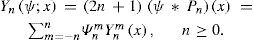
Note that each function ψx∈ℂ∞S is represented by its own Fourier-Laplace series ∑n=0∞ Ynψ; x and ψ2=∑n=1∞ Ynψ; x2.
Let s > 0 and ψx∈ℂ∞S. The derivative Λs = (–Δ)s/2 of real order s is defined as a multiplier operator, defined by infinite set of multiplicators χns/2n=1∞:

Besides,
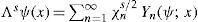
Obviously, operator Λs may be defined on functions from ℂ∞S=ψ∈ℂ∞ (S): Y0ψ = 0 by means of (4) for any real degree s. In particular, Λ2n = (−Δ)nfor a natural n, and operator Λ can be interpreted as the square root of nonnegative and symmetric Laplace operator. Unlike the local derivatives ∂n/∂λn and ∂n/∂μn, the derivatives Λs and projectors Yn are invariant with respect to any element of the group SO(3) of sphere rotations (Skiba, 2012).
3Hilbert spaces ℍsWe denote the completion of ℂ0∞S in norm (1) as the Hilbert space ℍ0=L02S= ⊕n=1∞Hn of functions on S. For any real s, we introduce the inner product •,•s, and norm||•||sin ℂ0∞S as


We denote the Hilbert space obtained by closing the space ℂ0∞S in norm (10) as ℍs. We will keep the symbols •,• and • for the inner product and norm in ℍ0. Let 0 < s < r. Then the imbeddings ℂ0∞S⊂ℍr ⊂ℍs ⊂ℍ0 ⊂ℍ−s ⊂ℍr are continuous, and the dual space ℍs* coincides with ℍ−s (Agranovich, 1965).
Let s and r be real numbers. Operator Λr = ℂ0∞(S) ↦ ℂ0∞(S) is symmetric, Λrψ,hs=ψ,Λrhs and hence, closable, and extended to ℍs. Namely, an element z ∈ ℍs is called the rth derivative Λrψ of a function ψ ∈ ℍs if z,hs=z,Λrhs holds for all h∈ ℂ0∞S (Skiba, 1989).
Lemma 1 (Skiba, 1989). Let s and r be real numbers, r > 0, and ψ ∈ ℍs+r. Then

Due to Lemma 1, the mapping Λr: ℍs+r ↦ ℍsis isometric and isomorphic for any real s and r. In particular, at r = –2s, the operator Λ−2s: ℍ−s ↦ℍs is an isometric isomorphism.
Lemma 2 (Skiba, 1989). Let r, s and t be real numbers, r

The dynamics of viscous and forced nondivergent barotropic fluid on the sphere S is described by the nonlinear barotropic vorticity equation

written in the geographical coordinate system (λ, μ) whose pole N is on the axis of rotation of the sphere (Skiba, 1969). Here ψ is the streamfunction, Δψ(t, x) is the relative vorticity, Δψ +2μ is the absolute vorticity, F(t, x) is the forcing, σΔψ describes the Rayleigh friction in the planetary boundary layer (σ ≥ 0),

is the Jacobian, J(ψ, 2μ) = 2ψλ describes the rotation of sphere, and n→ is the unit outward normal at a point of the sphere. The fluid velocity v→=n→×∇ψ is sole- noidal: ∇• v→ = 0. The turbulent viscosity term has the form ν(−Δ)s+1ψ, where v > 0 and s ≥ 1 is arbitrary real number (Skiba, 2012). As it was mentioned before, the value s = 1 corresponds to the classical viscosity term in Navier-Stokes equations (Szeptycki,1973a, b; Temam, 1984, 1985; Ladyzhenskaya, 1987; Ilyin and Filatov, 1988), s = 2 was considered in (Simmons et al., 1983; Dymnikov and Skiba, 1987a, b; Skiba, 1994), while natural numbers of s were used in (Lions, 1969) for proving the solvability of Navier-Stokes equations in a limited area by means of the method of artificial viscosity. Note that (14) is considered in the classes of functions, orthogonal to a constant on S, thus, Y0(ψ)=0 and Y0(F)=0.
We now briefly consider the main properties of Jacobian (15). Let all functions be complex-valued. It is clear that

Let n be a natural, and r be a real. Since ΛsYn(ψ) = χns/2 Yn(ψ), we get J(ψ, Λsψ) = 0 for any ψ ∈ Hn. Obviously, J(ψ, h) = 0 for any zonal functions ψ(μ) and h(μ). Also note that


and

holds for sufficiently smooth complex-valued functions ψ, g and h on S (Skiba, 1989).
Let ℂ be the set of complex numbers, ψ ∈ ℂ∞(S), ψ : S → C, and let Gψ=G∘ψ be a superposition of two functions. Then Jψ,ℍ,Gψ¯=0
Lemma 3 (Skiba, 2012). Let r be a real number, and ψ, h ∈ ℂ∞(S). Then

Lemma 4 (Skiba, 1989). Let ψ, h ∈ ℍ2 Then J(ψ, h) belongs to ℍ0 and
5Attractive set of BVE solutions
The existence and uniqueness of the weak solution to nonstationary BVE (14), as well as the existence of a weak solution of steady BVE were proved in Skiba (2012). A condition for the uniqueness of the steady solution was also given in Skiba (2012). Besides self-interest, the analysis of classes of functions, in which there exist BVE solutions is particularly important in the stability study of solutions.
We now consider particular forms of the forcing guaranteeing the existence in a phase space X of a bounded set B.
Theorem 1 (Skiba, 2013). Let s ≥ 1 in (14) and let F(x) ∈ ℍr be a steady forcing where r ≥ –1. Then every solution ψ(t, x) of BVE (14) will eventually be attracted by a bounded set B ⊂ X Moreover,

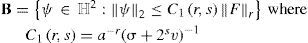


Here a=2 is the constant from Lemma 2.
Remark 1. All the steady and periodic solutions (if they exist) belong to the set B. Obviously, the set B contains the maximal attractor of the BVE (Temam, 1985).
Remark 2. If F(t, x) is a periodic forcing of space C(0, ω; ℍr) where ω is the time period, then Theorem 1 is also valid with the obvious change of the norm Fr by the norm maxt ∈ [0, ω]Fr
We now show that under certain conditions on the forcing and dissipation, the maximal attractor of BVE (9) coincides with the zero solution.
Theorem 2. If forcing F(t, x) is such that the integral ∫0∞||F(t,x)||rdt converges then ||ψ(t)||x→ 0 as t → ∞. Besides, X = ℍ2 if r ≥ 0 and X = ℍ1 if –1 ≤ r < 0.
Proof. Consider only the case Ft,x∈ℍr where r ≥ 0, since the case Ft,x∈ℍr where r ∈ [−1,0) is proved similarly. Taking the inner product of Eq. (9) with Δψ and using Lemma 3 we get

With lemmas 1 and 2, the terms F,Δψ and ν ||Λs+2ψ||2 can be estimated as

where a=2, and
Then (19) implies

Integrating (20) with respect to t from τ to t we obtain

where ||ψ||2 = ||Δψ|| (see [6] and [7]). Multiplying (20) by ||Δψ|| and integrating the result with respect to t from τ to t, we obtain

Estimating the norm ψt′2 in the r.h.s. of the last inequality with the help of (21) we get


Here we have 0≤τ≤t≤T. Hence, if integral ∫0∞||F(t,x)||r dt is finite then integral ∫0∞||ψ||22 dtis also finite. Therefore, there exists a subsequence tk → ∞ such that ψtk2→0 Using (21) in the case when τ = tk we obtain thatψt2→0 as t → ∞. The theorem is proven.
6Positive functional for the stability studyWe now introduce a positive functional related with kinetic energy and enstrophy of perturbations and derive an equation describing its behavior in time. Examples are given for the meteorologically important flows having the form of a super-rotation flow, a homogeneous spherical polynomial of degree n or a Rossby-Haurwitz wave.
Let ψ˜;(t, λ, μ) be a solution to BVE (9) under consideration, and let ψˆ(t, λ, μ) be another solution of (9). Then

wheres≥1, ν>0, and σ≥0, holds for the perturbationψ(t, λ, μ) = ψˆ (t,λ, μ) − ψ˜;(t, λ, μ) of ψ˜;. Taking the inner product (1) of Eq. (22) successively with ψ and Δψ and using the relations (14) and Lemma 3, we obtain two integral equations:
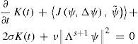

for the kinetic energy K(t) =12∇ψ2 and enstrophy η(t) =12Δψ2of the perturbation, respectively.
It follows from (23) and (24) that the Jacobian Jψ,Δψ˜; in (22) can change the perturbation enstrophy η(t) but does not affect the perturbation energy K(t). On the contrary, the other Jacobian Jψ˜;,Δψ in (22) has no effect on η(t) but can change K(t). As for the last two terms in the l.h.s. of (22) (the super-rotation term and the non-linear term), they both have no influence on the behavior of K(t) and η(t).
Example 1. If ψ˜; = 0 (such a solution exists if F(x) = 0) then Jψ,Δψ,ψ˜;)=0 and Jψ,Δψ,Δψ˜;)=0in (23) and (24). Therefore, in the non-dissipative case (σ = μ = 0), the zero solution is stable, since the perturbation energy and enstrophy will be constant. In a dissipative case σ≠0 and/or μ≠0 the zero solution is globally asymptotically stable, since the perturbation energy and enstrophy will exponentially decrease in time.
Let now ψ˜; be a solution of (9), and let p and q be non-negative numbers, not equal to zero simultaneously. We will measure the magnitude of perturbation with the functional
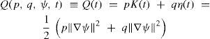
Multiplying (23) and (24) by p and q, respectively, and combining the results, we obtain

where

Lemma 2 leads to −Λs+1ψ2 ≤ −2s∇ψ2 and −Λs+2ψ2 ≤ −2sΔψ2, and hence (26) can be estimated as

Example 2.Super-rotation basic flow. Let ψ˜; = ψ˜;(μ) ≡ Cμ where C is a constant. Then R(t) = 0 due to (15) and Q(p, q, ψ, t) is the Liapunov function. Thus the super-rotation flow is Liapunov stable if σ = μ = 0, and is the global attractor (asymptotically Liapunov stable) if ρ>0. The same is true for any flow from subspace H1 (Skiba, 1989).
Example 3.Flow in the form of a homogeneous spherical polynomial. Let ψ˜;t,x∈Hn for some n ≥ 2, that is,

In particular, it can be a zonal Legendre-polynomial flow: ψ˜;(μ) = CPn (μ). Then J(ψ, Δψ) = 0 for any perturbation of Hn, and R(t) = 0. By (22), any perturbation of Hn will never leave Hn, that is, Hn is invariant set of perturbations to flow (29); besides, due to (28), Qp,q,ψ,t ≤ Qp,q,ψ,0 exp−2ρt. Thus any initial perturbation of Hn will exponentially tend to zero with time not leaving Hn, that is, set Hn belongs to the domain of attraction of solution (29).
Example 4. The basic flow ψ˜; is a linear combination of the flows considered in examples 2 and 3. In particular, ψ˜;(t, λ, μ) can be a Rossby-Haurwitz wave (Skiba, 1989, 2004).Then the result obtained in example 3 is also valid in this case.
7Evolution of functional Q(p, q, ψ, t)Eq. (22) for a perturbation ψ˜;t,x of solution ψ˜;t,x can be written as

where
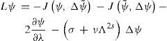
is a linear operator that has a compact resolvent ifv > 0 (Skiba, 1989, 1998). Using the Lagrange identity for defining the adjoint operators, Eq. (26) can be written as
where

is the symmetric operator in the space ℍ0.
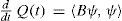
Let ωnandGn(x) be eigenvalues and orthonormal eigenfunctions of the spectral problem

Note that functions Gn(x) represent the orthonormal basis in the real space ℍ0, and operator B :ℍ0 → ℍ0 also has a compact resolvent (v > 0) and ωn are real isolated eigenvalues of geometrical multiplicity one. The only possible limit point of the spectrum is ω = −∞. Thus the number of positive eigenvalues of B is finite.
Let us now renumerate the eigenvalues {ωn} of operator B in such a way that their values are decreasing with increasing values of n. Besides, assume that the first N eigenvalues ω1,..., ωn are positive. The streamfunction of a perturbation ψt, x can be represented by its Fourier series

As a result we obtain

Assume that an initial perturbation ψ(t0, x) has the form of a single eigenfunction Gn(x): ψ(t0, x) = an(t0)Gn(x), then
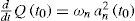
Therefore, if ωn>0 (or ωn<0) the functional Q(t) of such initial perturbation will increase (decrease). Note that the growth (decay) rate of Q(t) at the moment t0 is determined by the modulus of eigenvalue ωn and by the amplitude an(t0) of perturbation. In particular, if p = 1, q = 0 and all the eigenvalues are ordered so that ωn+1≤ ωn, then perturbation of the form of eigenfunction G1(x) will cause the fastest growth of the perturbation energy K(t).
Let us consider a sequence {an} of the Fourier coefficients of a perturbation (35) as a point in the phase space of perturbations to BVE solution ψ˜; (t, x). Then due to (36), the condition
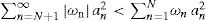
defines a subset ℳ0 in the coordinate space of points {an}. Any perturbation ψ, whose Fourier coefficients {an} belong to M0, generates the growth of Q(t).
It is interesting to study a structure of the set M0. Obviously, set M0 is unbounded because it includes the N-dimensional Euclidean space EN of vectors {a1, a2,..., aN} except for its origin {0, 0,..., 0}. The set ℳ0 is of infinite dimension and is not invariant with respect to applying the nonlinear operator Lψ − J(ψ, Δψ) of Eq. (22), that is, the trajectory of perturbation ψ(t, x) can enter and leave the set ℳ0. Obviously, among all the points {an} belonging to a surface ∑n=1N an2 = C = const the maximum of ddtQ(t) is achived when a1=C and an = 0 for all n ≥ 2.
It follows from (38) that if ∑n=1Nωn an2 is bounded then ∑n=N+1∞|ωn| an2 is also bounded. Since |ωn| → ∞ to as n → ∞ (recall that the operator B has a compact resolvent), the inequality ∑n=N+1∞|ωn|an2< C defines a compact set in the coordinate space of sequences{an}n=N+1∞, which is orthogonal to the N-dimensional Euclidean space EN.
Thus, the nonlinear evolution process for perturbations can be described by the following way. Assume that at an initial moment t0 the perturbation ψ(t0, x) is such that an(t0) = 0 for all n > N, i.e. the point {an(t0)} ∈ EN. Then functional Q(t) will grow. Since EN is not invariant, nonzero coefficients an(t) for n > N will appear. Their growth will render the inequality (38) invalid, and the point {an(t)} will leave the set ℳ0. From this moment the functional Q(t) will decrease. Note that the larger the number of nonzero coefficients an(t) with n > N, the higher the possibility for the point {an(t)} to leave the set ℳ0.
Example 5.Super-rotation basic flow. Let ψ˜; ≡ψ˜;(μ) = Cμ where C is a constant. Then

Since Δ and ∂∂λ are commutative, the operator [2(C −1) − CΔ]∂∂λ is skew symmetric, and hence,

Thus, the spherical harmonics Ynm(x) (n= 1, 2, 3, ...; |m|≤n) are the eigenfunctions Gn(x) of operator B corresponding to the eigenvalues ωn =−(σ+νχns) (qχn2 + pχn) where χn = n(n + 1). Since ωn < 0 for all n, the set ℳ0 defined by (38) is empty and Q(t) → 0 in time for any perturbation of super-rotation flow ψ˜;(μ) = Cμ (see Example 2).
8Conditions for global asymptotic stabilityIn a limited domain on the plane, in the absence of linear drag, a condition for global asymptotic stability of a BVE solution was derived by Sundström (1969), provided that the solution has continuous derivatives up to the third order. In this section we give three sufficient conditions for the global asymptotic stability of smooth and weak BVE solutions (theorems 3-5). These conditions differ by the smoothness of basic solution. The first two conditions were proved in Skiba (2013). The first condition (Theorem 3) generalizes Sundstrom's result to a flow on a rotating sphere when the linear drag is also taken into account and s ≥ 1 in the turbulent term. However, in the general case, the solvability theorems (Skiba, 2012) do not guarantee the existence of the solution whose third or higher derivatives are continuous. Therefore in the second condition (Theorem 4), the restriction on the smoothness of basic solution is weakened (only continuous derivatives up to the second order are required) and is in full accordance with the solvability theorems. The third condition (Theorem 5) is proved in this section for a weak BVE solution. Examples are given for a homogeneous spherical polynomial of subspace Hn and a pure dipole modon.
First, consider a rather smooth basic solution ψ˜;(t, x) of BVE (9) that has continuous derivatives up to the third order, so that
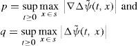
are both finite. Let us estimate the inner product (27) by means of functional (25) with p and q defined by (39):
Then substitution of (40) in (28) leads to
Theorem 3 (Skiba, 2013). Let s ≥ 1, v > 0 and σ ≥ 0. If a solution ψ˜;t,x of Eq. (9) is such that the numbers p and q defined by (39) are finite, and
then Q(p, q, y, t) is the Liapunov function, besides any perturbation of ψ˜;t,x will exponentially decrease in time.
In the particular case when s = 1 and σ = 0, Theorem 3 is analogous to the assertion (Sundström, 1969; Yu, 2005) for the flows in a limited domain on the plane. Note that both results demand the uniform boundedness of |∇Δψ˜;(t, x)| and |∇ψ˜;(t, x)|. However, the existence of BVE solutions is proved only in the classes of twice continuously differentiable stream- functions (Skiba, 2012). It was shown in Skiba (2013) that the restriction on the smoothness of solution could be weakened so as to be in accordance with the requirements of the solvability theorems.
Theorem 4 (Skiba, 2013). Let s ≥ 1, v > 0, σ ≥ 0, and let ψ˜;t,x be a solution of Eq. (9) such that numbers

defined by (42) are finite. If
then Q(p, q, y, t) is the Liapunov function, besides any perturbation of ψ˜;t,x will exponentially decrease in time.
Note that in contrast to Theorem 3, Theorem 4 requires a non-zero viscosity coefficient ν.
Unlike (39), condition (43) can be applied to a wider class of BVE solutions. For example, if ψ˜;t,x is a modon by Tribbia (1984), Verkley (1987) or Neven (1992), subjected to the linear drag and viscosity and supported by a certain forcing, then condition (43) is applicable, whereas (41) cannot be used because ∇Δψ˜;(t,x)is discontinuous on the boundary between the inner and outer regions of the modon.
Example 6. Let σ = 0 and s = 1 in Eq. (9), and let ψ˜;x be a stationary BVE solution from Hn (n ≥ 2):
This solution is supported by a steady forcing F(x) whose Fourier coefficients are equal to Fnm = (−νχn2 + i2m)ψ˜;nmwhere i=−1 and χn = n(n + 1). Due to Example 3, subspace Hn is the basin of attraction of solution ψ˜;x for any v. Besides, (42) leads to p = χnq, and by Theorem 4, solution (44) is the global attractor if ν≥q nn+1/2. Thus, the larger the velocity and degree n of flow (50), the larger must be the viscosity coefficient v to provide its global asymptotic stability.
Example 7.Pure dipole modon. Let us now specify condition (43) for the pure dipole stationary modon by Verkley (1987) provided that σ = 0 and s = 1 in Eq. (9). Such a modon has the form

in the local coordinate system (λ’, μ’), besides,

in the inner region Si=λ′,μ′∈S:μ′>a, and

in the outer region So=λ′,μ′∈S:μ′

for the stationary modon (43). In the relations (45)–(47), μ is the sine of latitude in the geographical system (λ, μ) whose pole μ = 1 is on the axis of rotation of sphere, and χα and χσ are the eigenvalues of the spherical harmonics used in constructing the modon in regions Si and So, besides, χα > 0 and χσ is a real. Note that p ≤ max {χα, | χσ |}q + 2, where q is defined by (42). As a result, condition (43) for the global asymptotic stability of modon explicitly depends on χα, | χσ| and q: ν2≥qq2maxχα,|χσ|+1.
We now derive a condition for the global asymptotic stability of a steady weak solution ψ˜;(x) ∈ℍs+2 s≥1, whose existence is proved in (Skiba, 2012).
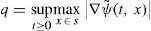
Theorem 5. Let s ≥ 1, v > 0 and σ ≥ 0. A steady weak solution ψ˜;(x) ∈ℍs+2 of BVE (9) is globally asymptotically stable if
where p=C0Δψ˜;L4S=∫SΔψ˜;4 dS1/4 and q=C0ψ˜;L4, and C0 is the constant from the estimate

(see lemmas 6 and 7 from Leray, 1933).
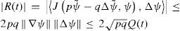
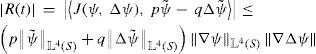
Proof. The functions ψ˜;(x) and Δψ˜;(x)belong to L4(S) due to lemma 4 from Leray (1933), and applying Hölder's inequality to (27) we get
Integrating the last inequality and applying (49) we obtain
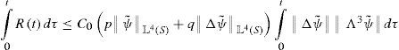
Setting p=C0Δψ˜;L4S and q=C0ψ˜;L4S and using ε-inequality, we get
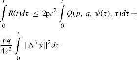
The integration of Eq. (26) in time and the use of the inequalities −||Λs+1ψ||2≤−2s||∇ψ||2 and −Λs+2ψ2≤−2s−1Λ3ψ2 lead to

with ρ = σ + 2sv. Applying (50) in (51) we obtain

The last term in this inequality is eliminated by setting ε2 = p/(2s+1v). Thus, ψ˜;x is globally asymptotically stable if ρ – pε2 > 0. The theorem is proved.
Remark 3. The restriction on the coefficient v weakens when the order s in the turbulent term of Eq. (9) increases. Also note that although the number q is absent in (48), it is present implicitly through the definition of functional Q(p, q, ψ, t).
9Hausdorff dimension of spiral attractor for a quasi-periodic forcing of Hn9.1Hausdorff dimension of BVE attractor subjected to a stationary forcingEstimates of the Hausdorff dimension of attractor in a viscous incompressible 2D fluid subjected in the periodic hypercube to a stationary forcing were made in Babin and Vishik (1989) and, in the more general case, in Constantin et al. (1988), Doering and Gibbon (1991), and Gibbon (1996). They state that the attractor dimension is limited by the nondimensional generalized Grashof number (Temam, 1984, 1985). In the case of sphere, the Hausdorff dimension of attractor of vorticity equation

was estimated in Ilyin (1994) as

where εG(s) → 0 as G(s) → ∞, and G(s) is the generalized Grashof number

and

is the L2-norm of the stationary forcing, and Fnm is its Fourier coefficient with respect to the orthonormal set of spherical harmonics Ynm(x) of the zonal number m and degree n ≥ 1. In particular, the inequality (52), as applied to large-scale barotropic processes of the atmosphere for s = 2 and G(2) = 1500, yields the upper limit of the barotropic atmosphere attractor dimension (Ilyin, 1994):

Despite the fact that the results (52) and (55) are of considerable theoretical interest in hydrodynamics, their practical application to the barotropic atmosphere raises doubts. Indeed, the forcing of the BVE (9) describes the influence of nonstationary small-scale baroclinic processes with rather complicated spatial and temporal behavior. So it is natural to expect that in contrast to stationary functions, small-scale quasi-periodic functions more adequately represent the BVE forcing.
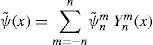
9.2Quasi-periodic spiral solutionIn order to show that the Hausdorff dimension of attractive sets crucially depends on the spectral composition of BVE forcing, we now consider the asymptotic behavior of solutions to the BVE (9) for a forcing which is quasi-periodic in time and has the form of a homogeneous spherical polynomial of degree n:

where

i is the imaginary unit, fm is a constant amplitude, and the numbers ωm are some incommensurate fundamental frequencies. Obviously, the geometric scale of forcing decreases as n increases. Note that the spherical variant of the well-known example by Marchioro (1986) corresponds to the time-independent forcing (56) of degree n = 1. Also note that the norm

of forcing (56), (57) is time-independent, and we will use the same generalized Grashof number (53) as in the case of stationary forcing. Obviously, there is a host of quasi-periodic forcings (56) that have the same norm (58) (or the same Grashof number [53]), but differ in their degrees n and amplitudes fm.
Due to (2) and (11), J(ψ, Δψ) = 0 for any ψ∈Hn, and hence, Hn is the invariant set of BVE solutions: any solution of (9) that starts in Hn will never leave Hn. Moreover, it follows from (27) that R(t) 0, and by (26), the subspace Hn is the attraction domain for the solution ψ˜;mt,x∈Hn defined by its Fourier coefficients (Skiba, 2013):

Since the frequencies ωm are rationally independent, the attractive solution ψ˜;t,x is quasi-periodic, and its path is an open (endless) spiral densely wound around a 2n-dimensional torus in the (2n + 1)- dimensional complex subspace Hn. According to theorem 3 by Samoilenko (1991), the closure of this trajectory coincides with the torus. Hence, the Hausdorff dimension of attractive solution (59) equals 2n.
9.3Global asymptotic stability of spiral solution (59)Sufficient condition for the global asymptotic stability of solution (59) is given by Theorem 3. In our case ψ˜;(t,x) ∈Hn, and (39) leads to p = χnq = n(n + 1)q. As a result, the condition (41) for global asymptotic stability of solution (59) accepts the form
where
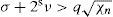
It is easy to show (see Skiba, 1994, Appendix B) that

According to (59) we have ψ˜;(t,x)≤σ+νχns−1 × χn−1F where ||F|| is the time-independent norm (58) of forcing (56). Using the last estimates in (61) we get

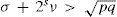
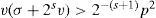
where bn(2n+1)/4π σ+νχns−1 and hence, condition (60) is satisfied if σ + 2sv > bn ||F|| and even more so if
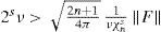
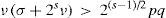
Using (53), condition (62) can be written in terms of generalized Grashof number: 22−sχnsπ/2n+1>Gs, and hence, it is satisfied if

Thus, we have proved the following assertion:
Theorem 6. Let s≥v>1,v>0,σ≥0,Ft,x∈Hn be a quasi-periodic BVE forcing (56), and let G(s) be the generalized Grashof number (53) of this equation. Then solution (59) of Hn is globally asymptotically stable provided that inequality (63) is fulfilled. Moreover, for a fixed finite Grashof number G(s), there is an integer nG so that for any n ≥ nG, the spiral solution generated by any forcing (56) of Hn with Grashof number G is globally asymptotically stable.
In particular, solution (59) is globally asymptotically stable if 21/2π n7/2 > G2 and 21/2π n3/2 > G1. The last case corresponds to the Navier-Stokes equations. For example, the condition 21/2π n7/2 > G2 is satisfied for any forcing (56) of degree n ≥ 8 if G(2) = 1500.
The result obtained is not unexpected. Indeed, for a fixed coefficient v(s), the number G(s) is fixed if the L2-norm (58) of the forcing is a constant independent of n. The amplitudes |fm| of forcing must decrease as n grows, and for n large enough (or for the amplitudes |fm|small enough) the viscosity v(s) is sufficient to make the quasi-periodic solution (59) globally asymptotically stable.
Thus, whereas the Hausdorff dimension of the BVE attractor subjected to a stationary forcing is limited above by the generalized Grashof number G (Ilyin, 1994), the Hausdorff dimension 2n of globally attractive spiral solution (59) may become arbitrarily large as the degree n of quasi-periodic forcing (56) grows. This result has a meteorological interest, since it shows that the dimension of the global attractor in the barotropic atmosphere crucially depends on the spatial and temporal structure of BVE forcing and it can be unlimited even if the Grashof number (53) is bounded.
Remark 4. For a steady forcing Ft,x∈Hn, condition (63) guarantees the global asymptotic stability of the steady BVE solution ψ˜;t,x∈Hn as well.
10ConclusionsThe nonlinear barotropic vorticity equation (BVE) describing the vortex dynamics of viscous incompressible and forced fluid on a rotating sphere is considered. It takes into account the Rayleigh friction, the rotation of sphere, the external vorticity source (forcing) F(t, x), and the turbulent viscosity term of common form v(–Δ)s+1ψ, where Δ is the spherical Laplace operator and s ≥ 1 is a real number.
The large-time behavior of its solutions is studied. Specific forms of steady BVE forcing have been found which guarantee the existence of a limited set that eventually attracts all the BVE solutions (Theorem 1). Additionally, theorem 2 shows that under certain conditions on the nonstationary forcing, the maximal BVE attractor coincides with the zero solution. Thus, the asymptotic behavior of BVE solutions depends on both the structure and the smoothness of forcing. Three sufficient conditions for the global asymptotic stability of BVE solutions of different degree of smoothness are also given (theorems 3-5).
Simple attractive sets of the BVE (9) subjected to a quasi-periodic forcing of subspace Hn of homogeneous spherical polynomials of degree n are analyzed. Each such set is a spiral quasi-periodic BVE solution densely wound on a 2n-dimensional torus in Hn. The Hausdorff dimension of its trajectory equals to 2n. As the generalized Grashof number G becomes small enough then the basin of attraction of such spiral solution is expanded from Hn to the entire BVE phase space. It is shown that for a given G, there exists an integer nG such that each spiral solution generated by a forcing of Hn with n ≥ nG (and Grashof number G) is globally asymptotically stable (Theorem 6). Thus, whereas the Hausdorff dimension of global attractor of the BVE subjected on a sphere to a stationary forcing is limited by Grashof number G, the Hausdorff dimension of globally attractive spiral solution (59) may become arbitrarily large as the degree n of quasi-periodic forcing (56) grows. Unlike a steady forcing, a quasi-periodic forcing more adequately describes the effects of small-scale baroclinic processes in the BVE, and therefore the last result is of meteorological interest, showing that the dimension of the global BVE attractor can be unlimited even if the generalized Grashof number is limited, and hence, the global attractor dimension crucially depends not only on the magnitude but also on the spatial and temporal structure of forcing. This also shows that the search of a finite-dimensional global attractor in the barotropic atmosphere is not well justified.