


En este trabajo se evalúa la calidad de las predicciones meteorológicas del modelo numérico de alta resolución Weather Research and Forecasting (WRF). Las condiciones iniciales y de frontera fueron obtenidas del modelo numérico de predicción meteorológica regional Consortium for Small-scale Modeling (COSMO) con resolución horizontal de 7km. El modelo WRF fue integrado durante enero y julio de 2013 en dos resoluciones horizontales (3 y 1km). Las predicciones numéricas del modelo WRF se evaluaron utilizando diferentes medidas estadísticas calculadas para la temperatura a 2 m y para la velocidad del viento a 10 m. Los resultados han mostrado una tendencia del modelo WRF a sobreestimar los valores de los parámetros meteorológicos analizados en comparación con las observaciones.
The aim of this paper is to evaluate the quality of high-resolution weather forecasts from the Weather Research and Forecasting (WRF) numerical weather prediction model. The lateral and boundary conditions were obtained from the numerical output of the Consortium for Small-scale Modeling (COSMO) model at 7km horizontal resolution. The WRF model was run for January and July 2013 at two horizontal resolutions (3 and 1km). The numerical forecasts of the WRF model were evaluated using different statistical scores for 2 m temperature and 10 m wind speed. Results showed a tendency of the WRF model to overestimate the values of the analyzed parameters in comparison to observations.
Limited area numerical models for short range forecast can be used for various research and operational forecasting applications. Despite recent improvements in model resolutions and advances in physical parameterizations, there are still limitations to the predictability possibilities offered by a limited area numerical model. Many questions regarding the performance of limited area models are related to the increase of the horizontal resolution of limited area numerical weather prediction models for short-range forecasts (Mass et al., 2002). Because some features of topographic circulations may require a smaller grid spacing to realistically simulate crucial structures, forecasts from high-resolution limited area models can have a higher accuracy than the global models. This is a result of the finer computational grid on a regional area, detailed specification of terrain and more detailed description of physical processes (WMO, 2012).
Recent research has shown that forecast accuracy increases with the decrease of grid spacing. Various studies done by Cardoso et al. (2012) and Heikkila et al. (2011) showed that high-resolution simulations are required especially for complex terrain, despite the high computational costs of such simulations. Adlerman and Droegemeier (2002) and Bernadet et al. (2000) indicated that some processes such as strong convection can only be captured when the resolution of the numerical model is decreased below 2km. Evaluations done over extended periods of time (Nachamkin and Hodur, 2000) have proven that increasing the horizontal resolution of weather prediction models improves numerical forecasts especially for integration domains with complex topographic features.
However, several points must be taken into account when performing high-resolution numerical simulations. An important limitation of the meteorological models at very high resolution is the inaccuracy of the real terrain representation because the data supplied by the model generally have a coarser resolution than the simulation domains (Lupascu et al., 2015), while Atlaskin and Vihma (2012) suggest that over an almost flat terrain horizontal resolution is not a major factor for the accuracy of 2 m temperature. Moreover, studies such as Zhong and Fast (2003) and Zhong et al. (2005) suggest that even in high-resolution numerical weather prediction (NWP) simulations forecast errors can still be quite large. A study conducted by Schepanski et al. (2015) showed that the choice of initial and boundary data have a greater impact on NWP simulations than the model grid resolution. Apart from this, high-resolution numerical simulations can sometimes prove to be less efficient due to cost limitations. The higher the resolution of the model, the higher the computational costs and storage space required for such numerical simulations (Morton et al., 2010, 2011).
The evaluation of high-resolution numerical simulations is itself affected by the limited availability and spatial density of meteorological observations (Gego et al., 2005).
In order to assess the quality of a numerical forecast we compare it with the corresponding observation or a good estimate of the true outcome. Numerical forecast verifications offer information about the nature of numerical forecast errors, the accuracy of the numerical forecasts and their improvement over time. Recommendations for numerical forecast verification methodologies were made by Stanski et al. (1989), Nurmi (2003), Wilks (2005), Jolliffe and Stephenson (2012).
The purpose of this study was to evaluate the quality of the numerical weather forecasts of the Weather Research and Forecasting (WRF) model (Skamarock et al, 2008) integrated at high-resolutions, coupled with the Consortium for Small-scale Modeling (COSMO) regional model (Schättler et al, 2012), for two different seasons. Brief descriptions of the model configuration and setup as well as the statistical methods employed for this study are given in section 2. The results of the study and their implications are discussed in section 3. The paper ends with conclusions regarding the performance of the WRF model using initial and lateral boundary conditions from the COSMO model.
2MethodologyFor this study, the WRF model (version 3.4.1) with the ARW (Advanced Research WRF solver) as the dynamical core was run at 3km horizontal resolution, using topography data at 3 s (approximately 90 m) horizontal resolution. The topography data were obtained from the NASA Shuttle Radar Topographic Mission (SRTM, http://srtm.csi.cgiar.org/) database, which provides digital elevation data for over 80% of the globe. The data were entered in the WRF model for the studied domain, extending between 20.0-35.0° E and 40.0-50.0° N.
The physical parameterizations used for this study include the Yonsei University (YSU) planetary boundary layer scheme (Hong and Dudhia, 2006), the WRF Single-Moment 5-class microphysics scheme (Hong et al, 2004), the 5-layer thermal diffusion land surface scheme (Chen and Dudhia, 2001), the Rapid Radiative Transfer Model (RRTM) scheme for longwave radiation (Mlawer and Clough, 1997), and the Dudhia (Dudhia, 1989) short-wave radiation scheme.
The output of the Consortium for Small-scale Modeling (COSMO) model at 7km horizontal resolution (Schättler et al., 2012) was used as lateral and boundary conditions for the WRF numerical weather forecast model (Skamarock et al., 2008). The COSMO numerical model uses a rotated latitude/longitude grid. In order to use the output of the COSMO-7km model for running the WRF model, a series of interpolation methods from rotated latitude/longitude grid into regular latitude/longitude grid were necessary.
The evaluation was carried out for two months, one during winter (January 2013) and one in the summer (July 2013). The WRF model was integrated independently (no feedback between the two integrations) at two horizontal resolutions (3 and 1km), for a domain which covered the entire Romanian territory with 261 ’ 191 grid points (3km) and 787 ´ 568 grid points (1km), respectively (presented in Fig. 1, outlined in red). The model was run for a 30 h forecast period with a spin-up period of 6 h.
 and location of meteorological stations used for verification (black dots).")
In order to assess the quality of the numerical weather forecast of the WRF model with COSMO lateral and boundary conditions (00:00 UTC run), we analyzed the ability of the model to forecast 2 m temperature and 10 m wind speed. Monthly and daily mean error (ME) and root mean square error (RMSE) were computed for both WRF-3km and WRF-1km taking into account all 163 Romanian synoptic stations (Fig. 1, black dots) which offer a very good coverage of the Romanian domain. The scores were computed for different forecast time steps (00:00 UTC + 6 h, 00:00 UTC + 12 h and 00:00 UTC + 18 h). Also, in order to assess the ability of the WRF model to forecast the above mentioned parameters, scatter plots were used for a more detailed analysis of the correspondence between the forecasted values and the observations for 2 m temperatures and 10 m wind speed. The formulas for ME and RMSE are presented below in Eqs. (1) and (2), respectively (Stanski et al., 1989;Nurmi, 2003):


where Fi represents the forecasts, Oi are the corresponding observations and N is the number of events.
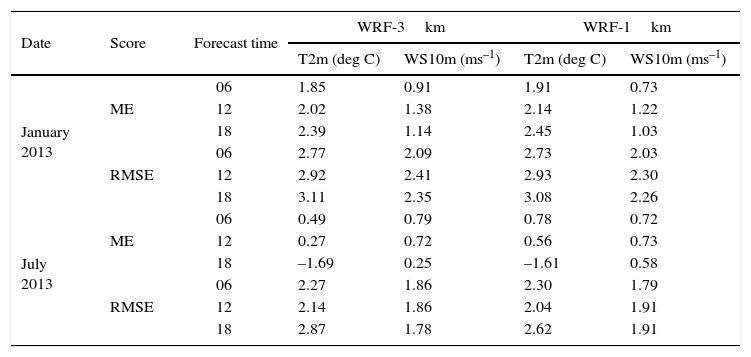
3Results and discussionThe general tendency of the WRF model to overestimate forecast values at both resolutions (3 and 1km) for 2 m temperature and 10 m wind speed in comparison with observations is also shown by the ME values for the two analyzed periods (Table I). As can be seen from ME values for 2 m temperature, the general tendency of both experiments (WRF-3km and WRF-1km) is to overestimate the forecasted values of this parameter in comparison with observations for the winter period analyzed. The same tendency can be noticed for the summer period for the 00:00 UTC + 6 h and for the 00:00 UTC + 12 h forecast. For the 00:00 UTC + 18 h forecast for the summer month, both models seemed to underestimate the values of the parameter in comparison with observations. For both months, differences in ME values between WRF-3km and WRF-1km vary between -0.06 deg C (for January 2013, 00:00 UTC + 6 h and 00:00 UTC + 12 h) and 0.29 deg C (July 2013, 00:00 UTC + 6 h and 00:00 UTC + 12 h). Despite the high values of RMSE for both months, errors of smaller amplitude can be noticed for WRF-1km than for WRF-3km for most of the analyzed period.
Two-meter temperature and 10 m wind speed mean error (ME) and root mean square error (RMSE) values for January 2013 and July 2013 (in deg C and ms1, respectively), for different time steps (00:00 UTC + 6 h, 00:00 UTC + 12 h and 00:00 UTC + 18 h), for both integration domains.
| Date | Score | Forecast time | WRF-3km | WRF-1km | ||
|---|---|---|---|---|---|---|
| T2m (deg C) | WS10m (ms–1) | T2m (deg C) | WS10m (ms–1) | |||
| January 2013 | ME | 06 | 1.85 | 0.91 | 1.91 | 0.73 |
| 12 | 2.02 | 1.38 | 2.14 | 1.22 | ||
| 18 | 2.39 | 1.14 | 2.45 | 1.03 | ||
| RMSE | 06 | 2.77 | 2.09 | 2.73 | 2.03 | |
| 12 | 2.92 | 2.41 | 2.93 | 2.30 | ||
| 18 | 3.11 | 2.35 | 3.08 | 2.26 | ||
| July 2013 | ME | 06 | 0.49 | 0.79 | 0.78 | 0.72 |
| 12 | 0.27 | 0.72 | 0.56 | 0.73 | ||
| 18 | –1.69 | 0.25 | –1.61 | 0.58 | ||
| RMSE | 06 | 2.27 | 1.86 | 2.30 | 1.79 | |
| 12 | 2.14 | 1.86 | 2.04 | 1.91 | ||
| 18 | 2.87 | 1.78 | 2.62 | 1.91 | ||
T2m: 2 m temperature; WS10 m: 10-m wind speed; ME: mean error; RMSE: root mean square error.
Daily ME and RMSE values were computed for WRF-3km and WRF-1km for the same forecast times mentioned above and are represented in Figs. 2–7. For 2 m temperature, slightly smaller daily error values can be noticed for WRF-3km compared to WRF-1km for most of January 2013. However, smaller amplitude of errors is generally obtained from WRF-1km for this period. Again, the tendency of the model to overestimate forecast values compared to observations is obvious for January 2013 for all analyzed forecast times (Figs. 2-4).
 and root RMSE (in black) in deg C for January 2013 (left) and July 2013 (right), 00:00 UTC + 6 h. WRF-3km (first row) and WRF-1km (second row).")
 and RMSE (in black) in deg C for January 2013 (left) and July 2013 (right), 00:00 UTC + 12 h. WRF-3km (first row) and WRF-1km (second row).")
 and RMSE (in black) in deg C for January 2013 (left) and July 2013 (right), 00:00 UTC + 18 h. WRF-3km (first row) and WRF-1km (second row).")
 and RMSE (in black) in ms–1 for January 2013 (left) and July 2013 (right), 00:00 UTC + 6 h. WRF-3km (first row) and WRF-1km (second row)")
 and RMSE (in black) in ms–1 for January 2013 (left) and July 2013 (right), 00:00 UTC + 12 h. WRF-3km (first row) and WRF-1km (second row).")
 and RMSE (in black) in ms–1 for January 2013 (left) and July 2013 (right), 00:00 UTC + 18 h. WRF-3km (first row) and WRF-1km (second row).")
For July 2013, the same behavior of overestimation can be noticed for the 00:00 UTC + 6 h forecast time, both for the WRF-3km and WRF-1km forecasts for most of the period (Fig. 2).
For the first part of the same period, the values of these scores computed for the 00:00 UTC + 12 h forecast time also show the same tendency to overestimate forecasted values of 2 m temperature compared to observations taking into account the WRF model integrated at both horizontal resolutions (Fig. 3). The analysis of ME and RMSE values for the same forecast time (00:00 UTC + 12 h) for the second part of July 2013, shows that WRF-1km and especially WRF-3km tend to underestimate forecasted values of this parameter in comparison to the observations from the meteorological sites (Fig. 3).
For the last forecast time analyzed here (00:00 UTC + 18 h, Fig. 4), the general tendency of the WRF model integrated at both horizontal resolutions is to overestimate forecasted 2 m temperature values compared to the observed ones for the entire month of January and to underestimate them for July. From Figure 3 it is also observed that the very small ME monthly value obtained previously for the 00:00 UTC + 12 h forecast time for July 2013 with the WRF-3km model was due to compensating errors (overestimation for the first half of the month and underestimation for the second half).
In Figures 5–7, 10 m wind speed daily ME and RMSE for January 2013 and July 2013 are represented for the three analyzed forecast steps (00:00 UTC + 6 h, 00:00 UTC + 12 h, 00:00 UTC + 18 h), for both WRF-3km and WRF-1km. It can be noticed that in a small number of cases, both models (WRF-3km in particular) forecasted smaller values for 10 m wind speed than the observed values for the 00:00 UTC + 18 h lead times (Fig. 7). Apart from these few cases, the general tendency of both WRF-3km and WRF-1km is to overestimate the values for this parameter compared to the observations for all forecast times analyzed.
In the scatter plots for 2 m temperature, forecast values are represented against the observed values (Fig. 8). As can be seen from Figure 8, at all forecast times during the entire period, many of the points represented are on or very close to the diagonal. The spread of the points shows a high accuracy of both WRF-3km and WRF-1km model forecasts for 2 m temperature. However, as previously seen from the ME and RMSE values computed for both models, the scatter plots show the same tendency of WRF- 3km and WRF-1km, that is, to overestimate the forecasted values in comparison to the observed ones for this parameter for January 2013 (all forecast times), July 2013 (00:00 UTC + 6 h forecast time) and the first part of July 2013 (00:00 UTC + 12 h forecast time) and underestimate them for the remaining period (00:00 UTC + 18 h) and the entire July period (00UTC +18 h).
 - January 2013 (first two rows) and July 2013 (last two rows), for different time steps (00UTC+6 h - left, 00:00 UTC + 12 h - center, 00:00 UTC + 18 h - right), for WRF-3km (first and third rows) and WRF-1km (second and fourth rows).")
Also, it can be noticed that the spread of the WRF-1km is slightly better than that for WRF-3km, especially in the case of the forecast for January 2013 and the 00:00 UTC + 12 h forecast for July 2013.
The scatter plots in Figure 9 show the spread of the forecast-observation errors for 10 m wind speed. The spread of the errors close to 0 indicate a high accuracy of both WRF-3km and WRF-1km in forecasting this parameter. A slightly greater spread of the errors as well as a stronger overestimation of the forecasted values vs. observations can be noticed for WRF-3km compared to WRF-1km. These results, as well as the ones shown above indicate a better performance from both WRF-3km and WRF-1km for the summer period analyzed in this study (July 2013) than for the winter period. It can also be noticed that for the same periods and forecast times the models have a similar behavior in that they both either underestimate or overestimate the values forecasted for 2 m temperature or 10 m wind speed in comparison with observed values.
. January 2013 (first two rows) and July 2013 (last two rows), for different time steps (00:00 UTC + 6 h - left, 00:00 UTC + 12 h - center), and 00:00 UTC + 18 h - right, for WRF-3km (first and third rows) and WRF-1km (second and fourth rows).")
Scatter plots for errors in 10 m wind speed (in ms–1). January 2013 (first two rows) and July 2013 (last two rows), for different time steps (00:00 UTC + 6 h - left, 00:00 UTC + 12 h - center), and 00:00 UTC + 18 h - right, for WRF-3km (first and third rows) and WRF-1km (second and fourth rows).
The purpose of this study is to evaluate the quality of the numerical weather forecasts of the WRF model integrated at two high resolutions.
The analysis of ME and RMSE for January 2013 and July 2013 indicate that the numerical weather forecast ofthe high-resolution WRF model for the 2 m temperature and 10 m wind speed parameters show differences depending on the forecast time and the horizontal resolution of the model.
For the present study, the WRF model was run with high-resolution topography data and lateral and boundary conditions from the limited area COSMO-7km model, using a standard configuration of the parameterization schemes available in the WRF model.
A first analysis of the results obtained in this study shows a good quality of the numerical forecasts from the WRF model integrated at high resolutions for Romanian territory.
The analysis of scatter plots for 2 m temperature and 10 m wind speed forecast from the WRF-3km and WRF-1km show a good correspondence between the model forecasts and the observed values for these parameters. This indicates a good accuracy of the model run at both horizontal resolutions, despite the general tendency of the WRF-3km and WRF-1km to overestimate the forecasted values in comparison to observations. It is also important to notice a similar behavior of WRF-3km and WRF-1km for the same periods and forecast times.
Results indicate a slightly better performance from the WRF-1km model compared to the WRF-3km model. Also, a better performance for both models can be noticed for the summer period analyzed in this paper.
Taking into account the model set-up employed in the present study, other improvements of the numerical weather forecasts of the high-resolution WRF model for Romanian territory can be further obtained by integrating this model using different parameterization schemes.