

This study investigates uncertainty levels of various industries and tries to determine financial ratios having the greatest information content in determining the set of industry characteristics. It then uses these ratios to develop industry specific financial distress models. First, we employ factor analysis to determine the set of ratios that are most informative in specified industries. Second, we use a method based on the concept of entropy to measure the level of uncertainty in industries and also to single out the ratios that best reflect the uncertainty levels in specific industries. Finally, we conduct a logistic regression analysis and derive industry specific financial distress models which can be used to judge the predictive ability of selected financial ratios for each industry. The results show that financial ratios do indeed echo industry characteristics and that information content of specific ratios varies among different industries. Our findings show diverging impact of industry characteristics on companies; and thus the necessity of constructing industry specific financial distress models.
In recent years financial ratio analyses have become popular managerial tools as well as tools for determining economic activity of firms. The ratios have gained acceptance even by small businesses for examining and describing the operations, and also by banks for making loan criticisms (Horrigan, 1968). They provide clarifications and insights into financial statements in making a variety of business decisions. In this regard, financial ratio analysis reduces uncertainty in decision making by providing a reliable assessment of the planning, operating, investing effectiveness and the health of financial activities of a businesses.
In the literature, a functional relationship between the financial ratios and some dependent variable of interest is estimated for prediction purposes. This type of models are mostly used by the investment analysts in estimating future profitability of a firm as well as by researchers in developing statistical models to predict failure of a company, to assess potential risks, to help with credit rating, etc. (Altman, 1968; Aziz et al., 1988; Beaver, 1966; Koh, 1992; Mossman et al., 1998; Ohlson, 1980; Taffler, 1983; Zmijewski, 1984). However, these or similar studies in the literature seldom took industry related factors into account, either by including control variables for industry effects or by constructing separate corporate failure prediction models for each industry to avoid inaccurate coefficient estimates. The sensitivity of bankruptcy prediction models to industry classifications (characteristics) raises the question of whether a single bankruptcy prediction model is sufficient to evaluate the financial conditions of firms in different industries. In other words, in the bankruptcy prediction models, whether using the same financial ratios for firms in different industries deteriorate the predicting ability of these models. Thus, this study aims to fill this gap in the literature by building industry specific financial distress models for certain industry groups sharing similar industry characteristics. Doing that, we aim to reduce the burden of information mass for the users of financial statements by limiting the number of financial ratios to those that have been found to have the greatest information content for each particular industry group.
To build industry specific financial distress models, we analyze information content of financial ratios in measuring the level of uncertainty of S&P 1500 firms in different industries to determine a set of industry specific financial ratios which possess the greatest amount of information for a specific industry. First, we chose 51 commonly used financial ratios and by use of factor analysis reduced them to several factors that account for the maximum variation in the data for the period 1990–2011. This technique further enables us to focus on the most stable and robust ratios between the sub-periods 1990–2000 and 2001–2011 by limiting the level of multicollinearity among the ratios. Second, following information theory perspective, we use the entropy method to find those financial ratios that provide more information on the level of uncertainty of firms within a particular industry group. The entropy method allows us to compute the probability distributions of perfect and imperfect information to determine the predictive ability of the information contained in the ratios for selected industries. The sensitivity of bankruptcy prediction models to industry classifications further raises the question of whether a single bankruptcy prediction model is sufficient to evaluate the financial condition of firms from different industries. Thus, after obtaining the set of financial ratios that possess the highest information content regarding the uncertainty level of firms within an industry group, we employ a logistic regression model to derive industry specific financial distress models. Finally, we examine the classification accuracy of these models in determining financially distressed companies.
Although there are studies that use entropy method in measuring information loss in the aggregation of accounting numbers (Theil, 1969; Lev, 1969) and that employ factor analysis of financial ratio patterns to examine stability of financial ratios over time and across countries (Yli-Olli and Virtanen, 1985, 1986), to our knowledge, no study has specifically analyzed the information content of financial ratios across industries. Moreover, few studies employ data reduction techniques in selecting financial ratios that are used in bankruptcy prediction models (Taffler, 1983). Thus, this study not only uses factor analysis as a data reduction technique but also employs the entropy method, as a second step, to examine the predictive ability and information content of the financial ratios derived from factor analysis. Finally, although there are considerable number of financial distress models in the accounting literature that predict company failure, most of these fail to capture industry characteristics and do not differentiate among distress probabilities in different industry groups. Therefore, our study serves as a first attempt distinguishing between distressed and non-distressed companies across industries; and in providing financial statement users with sharper tools to assess the probability of financial distress of firms in different industry groups.
This study consists of five sections. In Literature review section, we summarize the pertinent accounting literature: those that examine the information content of financial ratios in decision making; and those that build financial distress models which are commonly used in financial distress prediction. Next, we explain data and methodology and conduct factor analysis followed by entropy method to select the most informative financial ratios and derive financial ratio sets that are specific to each industry. In the following section, we report descriptive statistics and empirical outcomes along with necessary robustness checks. The final section is devoted to discussion and future research.
Literature reviewReducing set of financial ratios and determining their information contentA common goal of financial ratio analysis research is to derive the most useful financial ratios which provide substantial information about future events to be used in financial distress/bankruptcy models for prediction. Research on the determination of most useful financial ratios has largely focused on three main aspects: (i) stability of financial ratios over time, (ii) variations in financial ratios due to industry characteristics and (iii) obtaining a financial ratio set free from redundant information. To empirically determine the stability of financial ratios over time and the best information set, researchers employ factor analysis that start with an initial set of variables to obtain a smaller set of factors (combination of variables). They suggest that, financial ratios can be used in the financial distress/bankruptcy models if they show stable patterns of the factor values over time (Ezzamel et al., 1987; Pinches et al., 1973; Yli-Olli and Virtanen, 1985). Considering the second aspect, some researchers use factor and/or cluster analyses to identify industry specific differences and to determine variations among the financial ratios due to industry characteristics (Gupta, 1969; Gupta and Huefner, 1972; Johnson, 1979).
Because of the commonality of financial components within the financial ratios, the degree of overlap between those ratios with the same numerator or denominator becomes even greater, so much so that the additional information one ratio provides might be very small or even nil over another. Hence, taking into account the third aspect, selecting the most useful ratios, researchers use principal component analysis and/or canonical correlation analysis to separate redundant ratios from those that contain substantial information. This tends to limit the level of multicollinearity among the financial ratios (Chen and Shimerda, 1981; Laurent, 1979; Pohlman and Hollinger, 1981).
Overall, the literature reveals that factor analysis is a useful tool to manage a large set of exogenous variables, to compensate for random error and invalidity, and to disentangle complex interrelationships to derive major and meaningful linear combinations of variables that account for the maximum possible variation in the data.
To examine the information content of financial ratios and to investigate uncertainty level of companies, a remarkable number of researchers in accounting area use entropy method. In information theory, the method used to calculate the amount of uncertainty contained in a message is called entropy, a term first introduced by Shannon (1948). Theil (1969) uses entropy method in determining information content of accounting numbers and transforming accounting numbers into prior and posterior probabilities of total assets and liabilities for a particular accounting period. Theil also examines whether information content of aggregate versus disaggregate accounting numbers differ significantly. Similarly, Lev (1969) looking at the information loss caused by aggregation of accounting numbers, shows that the entropy of probability distribution of disaggregated accounts is greater than the entropy of probability distribution of aggregated accounts. Belkaui (1976) uses entropy method to measure asset, liability and balance sheet information and examines the ability of the information contained in these accounting numbers to predict a takeover event. Abdel Khalik (1974) employs entropy method in decision making, such as in loan granting decisions of commercial banks where the amount of information influences the decision to grant or deny credit. Finally, Peng et al. (2009), using entropy method, predict changes in the financial status of companies quoted in the Shanghai Stock Exchange. They examine financial ratios that have been shown in the literature to be correlated with financial crises and rank companies according to their entropy values. Overall, the literature on the entropy method in accounting points to the usefulness of the entropy method in strengthening the selection of most useful and informative ratios and their refinement.
Financial distress modelingIn this section, we review the prior literature on the financial distress/bankruptcy prediction models, and examine how studies define financial distress/bankruptcy; which financial ratios are preferred and included in the models and whether the models are powerful enough in predicting financial distress/bankruptcy. Since there is vast literature on financial distress/bankruptcy prediction models, we will limit the discussion by including only the most popular financial distress models.
Altman's (1968) bankruptcy prediction model is one of the most frequently cited bankruptcy prediction models in the literature. The ratios used in the prediction model are selected according to their popularity in the literature, including Working Capital/Total Assets (X1), Retained Earnings/Total Assets (X2), Earnings before Interest and Taxes/Total Assets (X3), Market Value of Equity/Book Value of Total Debt (X4) and Sales/Total Assets (X5). The author employing a multiple discriminant analysis (MDA) derives the following discriminant function:

The model predicts 95% of the total sample correctly one year prior to bankruptcy, while the accuracy rate falls to 72% two years prior to bankruptcy.
Ohlson (1980) derives a bankruptcy prediction model as an alternative to Altman's Z score model. The study employs logistic regression to examine the probability of a firm being bankrupt or non-bankrupt for the period of 1970–1976. The ratios used in the model are SIZE (logarithm of Total Assets/GNP Price Level Index), TLTA (Total Liabilities/Total Assets), WCTA (Working Capital/Total Assets), CLCA (Current Liabilities/Current Assets), OENEG (equals 1 if TL>TA and 0 otherwise), NITA (Net Income/Total Assets), FFOTL (Funds from Operations/Total Liabilities), INTWO (equals 1 if Net Income<0 for the last two years and 0 otherwise) and CHIN (change in Net Income) which are selected according to their frequent use in the literature. Ohlson's bankruptcy prediction model results in the following equation:
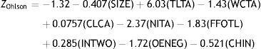
The logistic analysis shows that, the model correctly classifies 82.6% of the non-bankrupt and 87.6% of the bankrupt firms one year prior to bankruptcy.
Taffler (1983) formulates a bankruptcy prediction model for the manufacturing firms that are quoted in London Stock Exchange for the period, 1969–1976. The variables employed in the model are selected based on a factor analysis of potentially useful 80 ratios which results in 4 ratios that captures 91.6% of the total variance in the data set. Those ratios are PBT/AVCL (Profit Before Tax/Average Current Liabilities=X1), CA/TL (Current Assets/Total Liabilities=X2), CL/TA (Current Liabilities/Total Assets=X3) and No-Credit Interval ((Current Assets−Inventory−Current Liabilities)/(Sales−Profit Before Tax+Depreciation)=X4). Taffler runs a MDA model and obtains the following Z score model:
with a predictive accuracy of 95.7% for the bankrupt and 100% for the non-bankrupt firms.
Another popular financial distress prediction model is proposed by Zmijewski (1984) for the period, 1972–1978. A probit analysis, based on ROA (Net Income/Total Assets), FINL (Total Debt/Total Assets) and LIQ (Current Assets/Current Liabilities) as financial ratios resulted in the following model.

When Zmijewski uses matched sampling with unweighted probit analysis, the model classifies 92.5% of the bankrupt and 100% of the non-bankrupt firms correctly. Contrarily, when he does not use matched sampling, the classification accuracy falls to 62.5% for bankrupt and 99.5% for non-bankrupt firms.
Although there are numerous studies in the prior literature to predict financial distress/bankruptcy of firms, the question of how to predict financial distress of firms for different industries is still outstanding. For this reason, we propose to construct industry-specific financial distress models, using the most informative industry specific financial ratios that we derive based on factor analysis and entropy measures. The following section explains sample selection procedure, methodological design and model estimation process.
Data and methodologyDataData for this study are obtained from Datastream covering the period 1990–2011 on S&P 1500 firms that were active in the market as of March 2012. S&P 1500 firms include S&P 500, S&P Midcap 400 and S&P Smallcap 600 firms that make up approximately 90% of the U.S. market capitalization. 264 firms from the financial services are excluded as there are fundamental accounting differences between the financial services and other industries.
The firms belong to S&P 1500 classification covering information technology, industrials, healthcare, consumer discretionary, consumer staples, energy, materials, telecommunication services and utility industries. Since some of these industries show similar characteristics in terms of accounting practices, raw material usage and production process, we categorize firms into only 4 groups. First group “I1” covers firms in the consumer staples, consumer discretionary and health care industries. The second group “I2” includes firms in the energy and utility industries. The third group “I3” contains firms in the industrials and basic materials and the final group “I4” comprises of firms in the telecommunication services and information technology industries.
MethodologyFactor analysisIn this study, we employ 51 ratios that are selected from the existing literature after completing the two steps procedure (See Appendix A for the list of 51 ratios). First, we scan the financial ratio analysis literature, conducting factor analysis to determine the most informative ratios. Second, we select financial ratios which have 0.70 loadings or higher in these studies and eliminate those ratios that are very similar to each other in order to avoid redundant information and multicollinearity. After the selection procedure of 51 ratios, we conduct a factor analysis to determine a smaller set of variables from a large set that have special importance to the investigation (Anderson, 1963).1 To assess the overall significance of the correlation matrix and factorability of the overall set of variables Bartlett's test of sphericity and Kaiser–Meyer–Olkin (KMO) measure of sampling adequacy (MSA) are conducted. The results show that MSA values fall in the acceptable range (above 0.50) for all four industry groups. Likewise, Bartlett's test of sphericity is significant at 0.01% for all groups indicating appropriateness of the set of variables for factor analysis. Next, to select the most informative ratios, we look at the communalities of the variables in the un-rotated factor matrix and eliminate ratios with the communality levels of 0.50 or lower. We also derive anti-image correlation matrix of the variables to explore the individual MSAs and eliminate financial ratios that have MSA values under 0.50. Finally we examine the rotated component matrix to remove variables with factor loadings below 0.70; as well as those that load more than on one factor, since such variables do not have a significant contribution to explaining total variance of the factors. This procedure is conducted for each industry group.
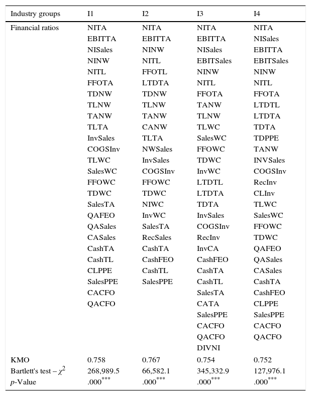
In factor analysis, the goal is to determine potentially “good” ratios and reselect among those that assess the same characteristics of the companies’ performance during changing cyclical conditions. Following the notion that a model is useful for prediction purposes only when the parameters and their association are stable over time (Seay et al., 2004), we examine the long term stability of financial ratios by dividing the sample into two sub periods: 1990–2000 and 2001–2011. To preserve stability of the ratios, we keep only those ratios that have factor loadings of at least 0.70 for both sub-periods.2 To see whether these ratios are stable over time, the procedure is repeated for each industry group. The reduced set of ratios for each industry group along with KMO and Bartlett's test of sphericity outcomes are presented in Table 1. It can be seen that these ratios preserve most of the information in the initial ratios and show stable patterns of factor solutions during the 22 year period relative to the excluded ratios in the data set.
List of selected financial ratios from factor analysis.
| Industry groups | I1 | I2 | I3 | I4 |
|---|---|---|---|---|
| Financial ratios | NITA | NITA | NITA | NITA |
| EBITTA | EBITTA | EBITTA | NISales | |
| NISales | NINW | NISales | EBITTA | |
| NINW | NITL | EBITSales | EBITSales | |
| NITL | FFOTL | NINW | NINW | |
| FFOTA | LTDTA | NITL | NITL | |
| TDNW | TDNW | FFOTA | FFOTA | |
| TLNW | TLNW | TANW | LTDTL | |
| TANW | TANW | TLNW | LTDTA | |
| TLTA | CANW | TLWC | TDTA | |
| InvSales | TLTA | SalesWC | TDPPE | |
| COGSInv | NWSales | FFOWC | TANW | |
| TLWC | InvSales | TDWC | INVSales | |
| SalesWC | COGSInv | InvWC | COGSInv | |
| FFOWC | FFOWC | LTDTL | RecInv | |
| TDWC | TDWC | LTDTA | CLInv | |
| SalesTA | NIWC | TDTA | TLWC | |
| QAFEO | InvWC | InvSales | SalesWC | |
| QASales | SalesTA | COGSInv | FFOWC | |
| CASales | RecSales | RecInv | TDWC | |
| CashTA | CashTA | InvCA | QAFEO | |
| CashTL | CashFEO | CashFEO | QASales | |
| CLPPE | CashTL | CashTA | CASales | |
| SalesPPE | SalesPPE | CashTL | CashTA | |
| CACFO | SalesTA | CashFEO | ||
| QACFO | CATA | CLPPE | ||
| SalesPPE | SalesPPE | |||
| CACFO | CACFO | |||
| QACFO | QACFO | |||
| DIVNI | ||||
| KMO | 0.758 | 0.767 | 0.754 | 0.752 |
| Bartlett's test – χ2 | 268,989.5 | 66,582.1 | 345,332.9 | 127,976.1 |
| p-Value | .000*** | .000*** | .000*** | .000*** |
This table presents the reduced set of financial ratios from the factor analysis for each industry group. It also shows the outcomes of KMO and Bartlett's test of sphericity. I1 includes firms in the consumer staples, consumer discretionary and health care industries, I2 includes firms in the energy and utility industries, I3 presents firms in the industrials and basic materials and I4 comprises of firms in the telecommunication services and information technology industries.
To discover industry specific financial ratios that possess the highest information content reflecting the uncertainty levels of these industry groups, we employ the entropy method as an information theory approach. The entropy method is a useful technique to determine the level of uncertainty of each industry group and to select industry specific financial ratios that best informs users of financial statements about the uncertainty level of firms belonging to a particular industry. This method is commonly used in multiple attribute decision making (MADM) to make preference decisions from a set of available alternatives that are differentiated by conflicting attributes. MADM is mainly used in the determination of appropriate weights for each criterion in the decision matrix. Both subjective and objective weighting schemes have been tried in the literature. In the MADM analysis, if the decision makers possess a priori weights for their preferences subjective weighting is used, whereas if such a priori weights do not exist, and the weights are computed from a mathematical model, weights are said to be objectively determined. The entropy method is one of such mathematical models used to determine objective weights when reliable subjective weights do not exist or difficult to obtain. It is also the most frequently used objective measuring technique in the decision making literature, since contrary to the other output models, it requires no distributional assumptions (Sobehart et al., 2001). Shannon's entropy is the most widely used technique in information theory to measure uncertainty, where the weight of an attribute decreases as the degree of entropy for that particular attribute increases (Lotfi and Fallahnejad, 2010). As the level of entropy increases, the discriminating ability of the attribute tend to decline, suggesting that, the weight for attributes with high entropy should be smaller, since decision makers would likely prefer those attributes with stronger discriminating power. In this manner, entropy measures the diversity of attribute values (Vetschera, 2000).
In information theory, Shannon (1948) suggested a probability function to represent the expected information content or entropy of a message, H as follows:
where pi is the probability of event i. In the above equation, if pk=1 for some k, and all other p=0 for i≠k then H, the entropy is minimum and equals zero corresponding to a case of certainty. On the other extreme, when all pis are probabilistically equal, 1/m, H reaches its maximum, Hmax and equals ln(m).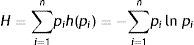
Although in the entropy literature, a variety of techniques have been used for the normalization of attribute values, a normalization formula developed by Zeleny (1974) has been used most frequently. In this model, the attributes are separated into two categories: those that increase entropy (impact negatively) and those that decrease (impact positively) it. In the literature, attributes that negatively affect entropy level are also classified as “cost type indices” and those that positively affect it are categorized as “benefit type indices” (Wang and Wang, 2012). However, in our study it is not possible to label the ratios as affecting the entropy level either positively or negatively, or as ratios that possess “benefit” or “cost” characteristic on the entropy levels of industries. It is because, up to a point, an increase in a financial ratio may be treated as a positive outcome while after an indeterminate limit, further increases might be considered negative. Moreover, this indeterminate level changes from company to company and from industry to industry. For reasons mentioned so far, we use the following formula in the normalization process of attribute values:
where xj*=maxxij,xjmin=minxij and consequently x is the jth ratio for the ith firm and rij measures closeness to the ideal solution where rij≥0 for every j. This is a one sided formula where all of the financial ratios are treated equally in terms of their effect on the entropy level. In other words, rij measures the distance of ratio j for company i from the minimum ratio j. Consequently, this one sided normalization method provides consistency among the outcomes in determining the entropy measure of importance.
The probabilistic outcomes of financial ratios can be defined as pij, and is computed by the following equation developed by Zeleny (1974):

Provided that pij determines the weights of importance for every financial ratio and pij≥0 for every i and j, the entropy Ej of the probabilistic outcomes of financial ratios is computed by the following equation:
where Ej represents the uncertainty or entropy of the message, and k=1/ln(m), positive constant guaranteeing t 0≤Ej≤1. Since entropy and uncertainty express the same concept, entropy of the probability distribution pi also represents the uncertainty of that probability distribution. According to information theory, probability estimates generated by financial ratio analyses are messages from an information system, and the amount of information in each message is computed by its ability to reduce uncertainty (Zavgren, 1985). Consequently, entropy is a decreasing function of the probability of an event.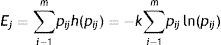
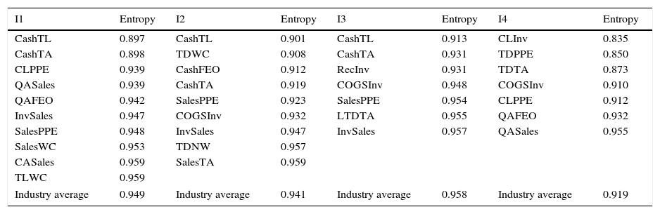
After normalization described above and computation of the entropy for every industry and each financial ratio which were selected by factor analysis, we obtain the entropy levels of the ratios and sort them in ascending order, where financial ratios with lower entropy levels possess more information on the uncertainty level of the industry groups. Table 2 lists financial ratios that have entropy scores below 0.96.3
Financial ratios selected by entropy method.
| I1 | Entropy | I2 | Entropy | I3 | Entropy | I4 | Entropy |
|---|---|---|---|---|---|---|---|
| CashTL | 0.897 | CashTL | 0.901 | CashTL | 0.913 | CLInv | 0.835 |
| CashTA | 0.898 | TDWC | 0.908 | CashTA | 0.931 | TDPPE | 0.850 |
| CLPPE | 0.939 | CashFEO | 0.912 | RecInv | 0.931 | TDTA | 0.873 |
| QASales | 0.939 | CashTA | 0.919 | COGSInv | 0.948 | COGSInv | 0.910 |
| QAFEO | 0.942 | SalesPPE | 0.923 | SalesPPE | 0.954 | CLPPE | 0.912 |
| InvSales | 0.947 | COGSInv | 0.932 | LTDTA | 0.955 | QAFEO | 0.932 |
| SalesPPE | 0.948 | InvSales | 0.947 | InvSales | 0.957 | QASales | 0.955 |
| SalesWC | 0.953 | TDNW | 0.957 | ||||
| CASales | 0.959 | SalesTA | 0.959 | ||||
| TLWC | 0.959 | ||||||
| Industry average | 0.949 | Industry average | 0.941 | Industry average | 0.958 | Industry average | 0.919 |
This table shows the most informative financial ratios that have entropy scores lower than 0.960 cut-off value, along with industry average entropy scores. I1 includes firms in the consumer staples, consumer discretionary and health care industries, I2 includes firms in the energy and utility industries, I3 presents firms in the industrials and basic materials and I4 comprises of firms in the telecommunication services and information technology industries.
Since in regression analysis each independent variable causes a loss of degree of freedom, having too many variables would result in an “over fitted” model with unrealistically high R2 (Babyak, 2004). In order to prevent this problem, in this study, we limit the number of variables by establishing a cut-off value for the acceptable entropy levels. It appears that after a value of about 0.96, the entropy values of the financial ratios do not change significantly. Therefore, we include only those ratios that meet this criterion of 0.96 in each industry model. This way, we avoid “over fitting” the models and preserve an adequate number of explanatory variables.
Logistic analysisAfter determining the most informative industry specific financial ratios, we employ logistic regression analysis to derive financial distress models for each industry group. In the literature, there are mainly two types of definitions regarding financially distressed firms. The first definition includes those firms that actually experience financial failure and are classified as failed by a legal declaration according to the bankruptcy law of the home country (Altman, 1968; Ohlson, 1980; Taffler, 1983; Zmijewski, 1984). The second definition includes those firms that have not declared bankruptcy yet, but experience financial difficulties which may arise from firm, industry c or even country specific factors (DeAngelo and DeAngelo, 1990; Smith and Graves, 2005; Li and Sun, 2008; Hill et al., 2011). Since our sample comprises of S&P 1500 firms that are active in the market as of March, 2012 when none of them had experienced bankruptcy yet, we use the second definition above: those that experience financial difficulty. Following the prior literature, firms experiencing financial difficulty are identified as those that had negative net income for at least 3 or 5 consecutive years between the periods 1990–2011 (DeAngelo and DeAngelo, 1990; Gilbert et al., 1990; Hill et al., 2011; Li and Sun, 2008; Mcleay and Omar, 2000). Since the study covers a period of 22 years, firms with at least 5 consecutive years of negative net income would be a rather accurate criterion by which a firm may be classified as in distress. However, in the energy and utility industry (I2), there are only two firms in the sample that satisfy this definition which precludes a logistic model due to insufficient sample size. To overcome this difficulty, in the energy and utility industry, we chose to classify firms as in distress if they had at least 3 consecutive years of negative income. Consequently 53 firms out of 414 in I1, 16 firms out of 139 in I2, 10 firms out of 283 in I3, and 33 firms out of 228 in I4 are classified as distressed firms.
In the logistic analysis, the binary dependent variable is the financial distress variable that takes the value one, if the firm is financially distressed and zero otherwise. The independent variables are those selected by the entropy method that have entropy scores lower than 0.96. We estimate logistic regression models for each industry group to test whether the most informative financial ratios selected by the entropy method can correctly classify financially distressed and non-distressed firms. Then, we generate industry specific financial distress models (FD models) using the coefficient estimates derived from the logistic analyses.
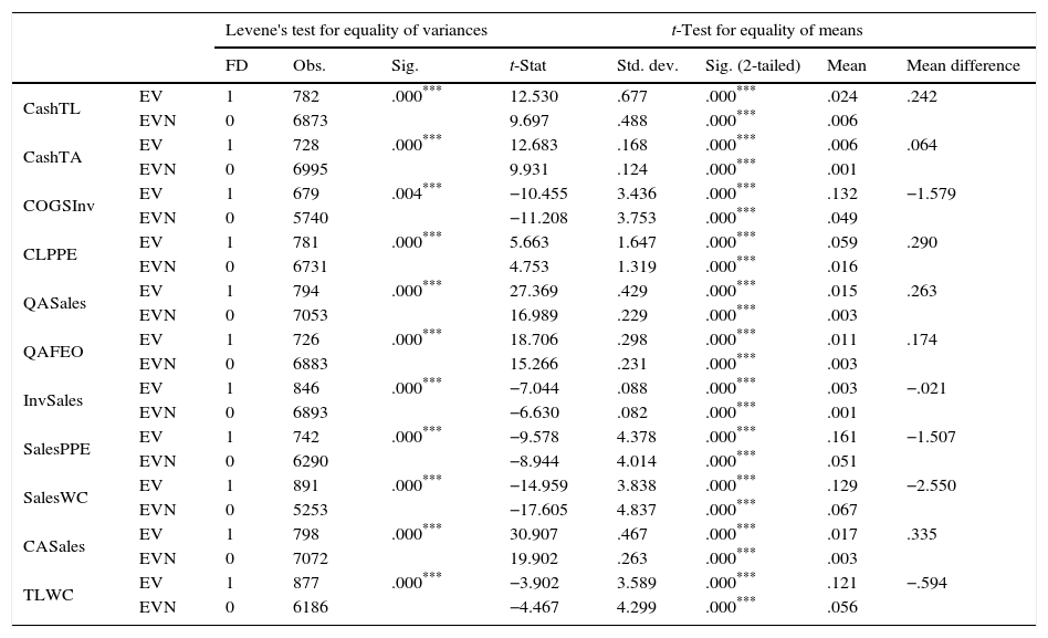
Descriptive statistics and empirical resultsPrior to the estimation of the logistic model, the Levene's test for equality of variances and t test for equality of means are conducted to examine whether the means and variances of industry specific financial ratios differed between the distressed and non-distressed firms. Tables 3–6 show the group statistics of financial ratios including means, standard deviations, t-statistics for equality of means and the Levene's test for equality of variances between distressed and non-distressed firms for I1, I2, I3 and I4 industry groups respectively.
Descriptives and independent sample test for I1.
| Levene's test for equality of variances | t-Test for equality of means | ||||||||
|---|---|---|---|---|---|---|---|---|---|
| FD | Obs. | Sig. | t-Stat | Std. dev. | Sig. (2-tailed) | Mean | Mean difference | ||
| CashTL | EV | 1 | 782 | .000*** | 12.530 | .677 | .000*** | .024 | .242 |
| EVN | 0 | 6873 | 9.697 | .488 | .000*** | .006 | |||
| CashTA | EV | 1 | 728 | .000*** | 12.683 | .168 | .000*** | .006 | .064 |
| EVN | 0 | 6995 | 9.931 | .124 | .000*** | .001 | |||
| COGSInv | EV | 1 | 679 | .004*** | −10.455 | 3.436 | .000*** | .132 | −1.579 |
| EVN | 0 | 5740 | −11.208 | 3.753 | .000*** | .049 | |||
| CLPPE | EV | 1 | 781 | .000*** | 5.663 | 1.647 | .000*** | .059 | .290 |
| EVN | 0 | 6731 | 4.753 | 1.319 | .000*** | .016 | |||
| QASales | EV | 1 | 794 | .000*** | 27.369 | .429 | .000*** | .015 | .263 |
| EVN | 0 | 7053 | 16.989 | .229 | .000*** | .003 | |||
| QAFEO | EV | 1 | 726 | .000*** | 18.706 | .298 | .000*** | .011 | .174 |
| EVN | 0 | 6883 | 15.266 | .231 | .000*** | .003 | |||
| InvSales | EV | 1 | 846 | .000*** | −7.044 | .088 | .000*** | .003 | −.021 |
| EVN | 0 | 6893 | −6.630 | .082 | .000*** | .001 | |||
| SalesPPE | EV | 1 | 742 | .000*** | −9.578 | 4.378 | .000*** | .161 | −1.507 |
| EVN | 0 | 6290 | −8.944 | 4.014 | .000*** | .051 | |||
| SalesWC | EV | 1 | 891 | .000*** | −14.959 | 3.838 | .000*** | .129 | −2.550 |
| EVN | 0 | 5253 | −17.605 | 4.837 | .000*** | .067 | |||
| CASales | EV | 1 | 798 | .000*** | 30.907 | .467 | .000*** | .017 | .335 |
| EVN | 0 | 7072 | 19.902 | .263 | .000*** | .003 | |||
| TLWC | EV | 1 | 877 | .000*** | −3.902 | 3.589 | .000*** | .121 | −.594 |
| EVN | 0 | 6186 | −4.467 | 4.299 | .000*** | .056 | |||
This table shows the Levene's test for equality of variances and t-test for equality of means for the I1 group. EV stands for the assumption of equality of variances and EVN stands for no assumption of equality of variances. FD refers to financial distress, where 1 stands for the distressed firms and 0 stands for the non-distressed firms.
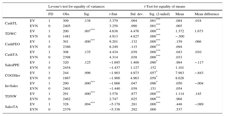
Descriptives and independent sample test for I2.
| Levene's test for equality of variances | t-Test for equality of means | ||||||||
|---|---|---|---|---|---|---|---|---|---|
| FD | Obs. | Sig. | t-Stat | Std. dev. | Sig. (2-tailed) | Mean | Mean difference | ||
| CashTL | EV | 1 | 309 | .138 | 3.379 | .094 | .001*** | .084 | .018 |
| EVN | 0 | 2405 | 3.258 | .090 | .001*** | .065 | |||
| TDWC | EV | 1 | 200 | .007*** | 4.638 | 4.476 | .000*** | 1.372 | 1.673 |
| EVN | 0 | 1481 | 4.913 | 4.827 | .000*** | −.300 | |||
| CashFEO | EV | 1 | 301 | .000*** | 9.201 | .132 | .000*** | .159 | .066 |
| EVN | 0 | 2386 | 8.249 | .115 | .000*** | .094 | |||
| CashTA | EV | 1 | 308 | .135 | 4.434 | .039 | .000*** | .043 | .010 |
| EVN | 0 | 2398 | 4.314 | .038 | .000*** | .033 | |||
| SalesPPE | EV | 1 | 320 | .125 | −1.695 | 1.400 | .090* | .984 | −.117 |
| EVN | 0 | 2454 | −1.437 | 1.127 | .152 | 1.101 | |||
| COGSInv | EV | 1 | 244 | .996 | −1.903 | 4.973 | .057* | 7.983 | −.643 |
| EVN | 0 | 1867 | −1.900 | 4.963 | .058* | 8.626 | |||
| InvSales | EV | 1 | 290 | .000*** | −1.666 | .047 | .096* | .050 | −.004 |
| EVN | 0 | 2401 | −1.440 | .039 | .151 | .054 | |||
| TDNW | EV | 1 | 291 | .000*** | 3.578 | .877 | .000*** | 1.114 | .145 |
| EVN | 0 | 2462 | 2.747 | .625 | .006*** | .968 | |||
| SalesTA | EV | 1 | 328 | .004*** | −5.178 | .281 | .000*** | .448 | −.089 |
| EVN | 0 | 2379 | −5.336 | .292 | .000 | .537 | |||
This table shows the Levene's test for equality of variances and t-test for equality of means for the I2 group. EV stands for the assumption of equality of variances and EVN stands for no assumption of equality of variances. FD refers to financial distress, where 1 stands for the distressed firms and 0 stands for the non-distressed firms.
Descriptives and independent sample test for I3.
| Levene's test for equality of variances | t-Test for equality of means | ||||||||
|---|---|---|---|---|---|---|---|---|---|
| FD | Obs. | Sig. | t-Stat | Std. dev. | Sig. (2-tailed) | Mean | Mean difference | ||
| CashTL | EV | 1 | 176 | .017** | 1.952 | .221 | .051* | .183 | .030 |
| EVN | 0 | 5322 | 1.757 | .198 | .081* | .153 | |||
| CashTA | EV | 1 | 180 | .393 | 1.491 | .083 | .136 | .085 | .009 |
| EVN | 0 | 5486 | 1.486 | .082 | .139 | .075 | |||
| RecInv | EV | 1 | 171 | .183 | −3.989 | 2.025 | .000*** | 1.172 | −.577 |
| EVN | 0 | 4741 | −3.670 | 1.851 | .000*** | 1.750 | |||
| COGSInv | EV | 1 | 163 | .915 | −4.748 | 2.929 | .000*** | 4.623 | −1.323 |
| EVN | 0 | 4463 | −5.623 | 3.514 | .000*** | 5.946 | |||
| SalesPPE | EV | 1 | 180 | .183 | −2.421 | 4.027 | .015** | 4.507 | −.776 |
| EVN | 0 | 5282 | −2.539 | 4.237 | .012** | 5.284 | |||
| LTDTA | EV | 1 | 180 | .000*** | 3.724 | .165 | .000*** | .229 | .039 |
| EVN | 0 | 5557 | 3.149 | .138 | .002*** | .190 | |||
| InvSales | EV | 1 | 153 | .000*** | 9.976 | .109 | .000*** | .179 | .066 |
| EVN | 0 | 5578 | 7.426 | .079 | .000*** | .113 | |||
This table shows the Levene's test for equality of variances and t-test for equality of means for the I3 group. EV stands for the assumption of equality of variances and EVN stands for no assumption of equality of variances. FD refers to financial distress, where 1 stands for the distressed firms and 0 stands for the non-distressed firms.
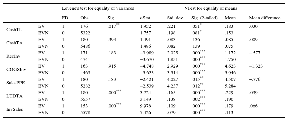
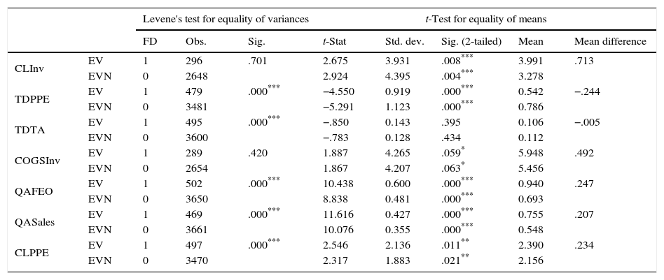
Descriptives and independent sample test for I4.
| Levene's test for equality of variances | t-Test for equality of means | ||||||||
|---|---|---|---|---|---|---|---|---|---|
| FD | Obs. | Sig. | t-Stat | Std. dev. | Sig. (2-tailed) | Mean | Mean difference | ||
| CLInv | EV | 1 | 296 | .701 | 2.675 | 3.931 | .008*** | 3.991 | .713 |
| EVN | 0 | 2648 | 2.924 | 4.395 | .004*** | 3.278 | |||
| TDPPE | EV | 1 | 479 | .000*** | −4.550 | 0.919 | .000*** | 0.542 | −.244 |
| EVN | 0 | 3481 | −5.291 | 1.123 | .000*** | 0.786 | |||
| TDTA | EV | 1 | 495 | .000*** | −.850 | 0.143 | .395 | 0.106 | −.005 |
| EVN | 0 | 3600 | −.783 | 0.128 | .434 | 0.112 | |||
| COGSInv | EV | 1 | 289 | .420 | 1.887 | 4.265 | .059* | 5.948 | .492 |
| EVN | 0 | 2654 | 1.867 | 4.207 | .063* | 5.456 | |||
| QAFEO | EV | 1 | 502 | .000*** | 10.438 | 0.600 | .000*** | 0.940 | .247 |
| EVN | 0 | 3650 | 8.838 | 0.481 | .000*** | 0.693 | |||
| QASales | EV | 1 | 469 | .000*** | 11.616 | 0.427 | .000*** | 0.755 | .207 |
| EVN | 0 | 3661 | 10.076 | 0.355 | .000*** | 0.548 | |||
| CLPPE | EV | 1 | 497 | .000*** | 2.546 | 2.136 | .011** | 2.390 | .234 |
| EVN | 0 | 3470 | 2.317 | 1.883 | .021** | 2.156 | |||
This table shows the Levene's test for equality of variances and t-test for equality of means for the I4 group. EV stands for the assumption of equality of variances and EVN stands for no assumption of equality of variances. FD refers to financial distress, where 1 stands for the distressed firms and 0 stands for the non-distressed firms.
The results show that all of the financial ratios have significantly different variances and means at 1% significance between distressed and non-distressed firms in the I1 industry group, while in the I2 SalesPPE, COGSInv and InvSales have different means only at 10% significance level. Moreover, CashTL and CashTA ratios possess equal variances with unequal means, while InvSales ratio possesses unequal variances but equal means. These results indicate that, the distressed and non-distressed groups differ either in terms of means values or in terms of standard deviations. In I3 group, we observe that RecInv, COGSInv, LTDTA and InvSales ratios have different means between distressed and non-distressed firms at 1% level of significance. Additionally, the mean values of SalesPPE and CashTL ratios also differ between groups at 5% and 10% significance levels respectively. Meanwhile, for CashTA ratio, both Levene's Test for equality of variances and t-test for equality of means shows that, neither the variance nor the mean differ between the groups. Finally, the results for I4 group show that CLInv, TDPPE, QAFEO and QASales ratios have different means between groups at 1% significance level, while CLPPE and COGSInv have different means between the groups at 5% and 10% level of significance respectively. Moreover, TDTA ratio possesses equal mean with unequal variances at 1% level of significance, while COGSInv and CLInv ratios possess equal variances with unequal means at 10% and 1% level of significance respectively. Results indicate that distressed and non-distressed groups differ at least in terms of group means or group variances.
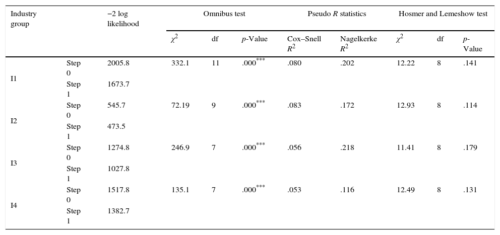
Results of logistic analysisLogistic Analysis provides two basic outcomes; predictive accuracy of the overall model and the significance of coefficients used in the model. Predictive accuracy of the model is determined by a classification matrix which indicates the type I and type II errors in classification accuracy of the individual groups (distressed and non-distressed firms) as well as, that of the overall model.4 In investigating the accuracy of the classification matrix and the overall model fit, we analyzed and checked Iteration History of the Base and the Estimated Model, Omnibus test, Hosmer and Lemeshow χ2 test, pseudo R statistics and −2 log likelihood values (the results are given in Appendix B).5 In estimating the logistic coefficients, we used Wald statistics and assessed the significance of each independent variable.6
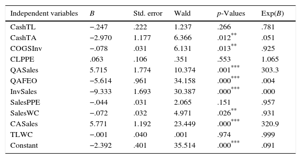
In the consumer staples, consumer discretionary and health industry group (I1), CashTL, CashTA, COGSInv, CLPPE, QASales, QAFEO, InvSales, SalesPPE, SalesWC, CASales and TLWC ratios are included as exogenous variables in the financial distress prediction model. Table 7 shows the classification matrix along with the coefficient estimates of the logistic regression. We observe that for both distressed and non-distressed groups, at a cut off score of 0.059 (which minimizes type I and type II errors) prediction accuracy of the model is considerably better than predicting by chance criterion, which is 50% for each group. Additionally, the analysis also shows that, the model correctly predicts distressed firms more accurately than non-distressed firms. Wald Test statistics reveal that, QASales, QAFEO, InvSales and CASales are statistically significant at 1%, while CashTA, COGSInv and SalesWC are at 5% in explaining the predicted probability of financial distress; however CashTL, CLPPE, SalesPPE and TLWC are not significant. We check whether dropping the insignificant variables from the model ameliorate the prediction accuracy or improve the overall fit of the model, but discover that, deleting any of the variables do not improve the models. When we look at the direction of the relationship between statistically significant ratios and financial distress, we observe that some of the ratios possess negative sign (their Exp(B) values are below) and some positive sign (their Exp(B) values are above 1). For e industry group I1 the results show that, CashTA, COGSInv, QAFEO, SalesWC and InvSales are negatively, while CASales and QASales are positively related to financial distress. In other words, as the values of either CASales or QASales increase, the predicted probability of financial distress also increases, which in turn increases the likelihood that a firm will be classified as distressed. Meanwhile, as the values of CashTA, COGSInv, QAFEO, SalesWC and InvSales increase, the likelihood that a firm will be classified as distressed will decrease.
Classification matrix and logistic analysis of I1.
| Independent variables | B | Std. error | Wald | p-Values | Exp(B) |
|---|---|---|---|---|---|
| CashTL | −.247 | .222 | 1.237 | .266 | .781 |
| CashTA | −2.970 | 1.177 | 6.366 | .012** | .051 |
| COGSInv | −.078 | .031 | 6.131 | .013** | .925 |
| CLPPE | .063 | .106 | .351 | .553 | 1.065 |
| QASales | 5.715 | 1.774 | 10.374 | .001*** | 303.3 |
| QAFEO | −5.614 | .961 | 34.158 | .000*** | .004 |
| InvSales | −9.333 | 1.693 | 30.387 | .000*** | .000 |
| SalesPPE | −.044 | .031 | 2.065 | .151 | .957 |
| SalesWC | −.072 | .032 | 4.971 | .026** | .931 |
| CASales | 5.771 | 1.192 | 23.449 | .000*** | 320.9 |
| TLWC | −.001 | .040 | .001 | .974 | .999 |
| Constant | −2.392 | .401 | 35.514 | .000*** | .091 |
| 0 | 1 | % Correctly predicted | |
|---|---|---|---|
| 0 | 2454 | 1247 | 66.4 |
| 1 | 59 | 217 | 78.6 |
| Overall | 2513 | 1464 | 67.2 |
This table presents the classification matrix and the logistic results of I1 industry group. Coefficients and exponential coefficients for financial ratios are represented by B and Exp(B) respectively. Standard errors, Wald test statistics are reported along with the corresponding p-values. The cut-off score for I1 is 0.059.
** Significance at .05 level.
*** Significance at .01 level.
I1 includes firms in the consumer staples, consumer discretionary and health care industries.
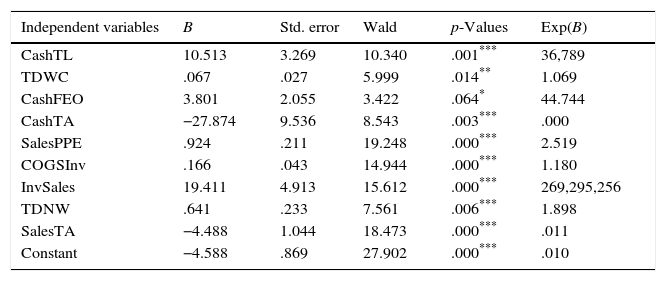
Table 8 shows the classification matrix and the logistic regression results for the energy and utility industry group (I2). CashTL, TDWC, CashFEO, CashTA, SalesPPE, COGSInv, InvSales, TDNW and SalesTA ratios are included in the financial distress model as independent variables. The outcomes show that, the model's overall correct classification percentage is 62.5%; specifically, the model correctly classifies 60.5% of the non-distressed and 81% of the distressed firms, based on a cut off score of 0.077. Similar to the outcomes of I1, classification accuracy of the model for I2 is greater in the distressed group than in the non-distressed group. When we consider the issue from the lenders’ point of view, higher prediction accuracy of distressed group is more useful, since misclassification cost of distressed firms would be greater due to failure to foresee non-payment risk. According to Wald Test statistics, CashTL, CashTA, SalesPPE, COGSInv, InvSales, TDNW and SalesTA are statistically significant at 1%, while TDWC and CashFEO at 5% and 10% respectively. B and Exp(B) values reveal that, CashTA and SalesTA are negatively, while CashTL, TDWC, CashFEO, SalesPPE, COGSInv, InvSales and TDNW are positively related to financial distress. The results show that, the likelihood that a firm is classified as distressed increases as the financial ratios with positive sign (CashTL, TDWC, CashFEO, SalesPPE, COGSInv and InvSales) increase, while the likelihood that a firm is classified as distressed decreases as the financial ratios with negative sign (CashTA and SalesTA) increase.
Classification matrix and logistic analysis of I2.
| Independent variables | B | Std. error | Wald | p-Values | Exp(B) |
|---|---|---|---|---|---|
| CashTL | 10.513 | 3.269 | 10.340 | .001*** | 36,789 |
| TDWC | .067 | .027 | 5.999 | .014** | 1.069 |
| CashFEO | 3.801 | 2.055 | 3.422 | .064* | 44.744 |
| CashTA | −27.874 | 9.536 | 8.543 | .003*** | .000 |
| SalesPPE | .924 | .211 | 19.248 | .000*** | 2.519 |
| COGSInv | .166 | .043 | 14.944 | .000*** | 1.180 |
| InvSales | 19.411 | 4.913 | 15.612 | .000*** | 269,295,256 |
| TDNW | .641 | .233 | 7.561 | .006*** | 1.898 |
| SalesTA | −4.488 | 1.044 | 18.473 | .000*** | .011 |
| Constant | −4.588 | .869 | 27.902 | .000*** | .010 |
| 0 | 1 | % Correctly predicted | |
|---|---|---|---|
| 0 | 456 | 298 | 60.5 |
| 1 | 16 | 68 | 81.0 |
| Overall | 472 | 366 | 62.5 |
This table presents the classification matrix and the logistic results of I2 industry group. Coefficients and exponential coefficients for financial ratios are represented by B and Exp(B) respectively. Standard errors, Wald test statistics are reported along with the corresponding p-values. The cut-off score for I2 is 0.077.
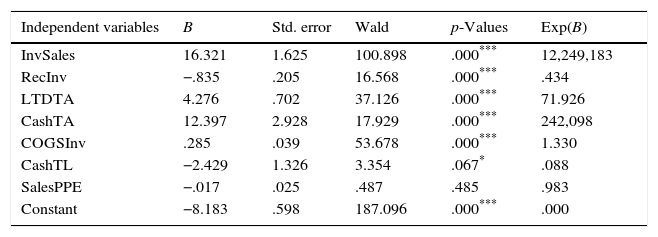
Table 9 exhibits the classification matrix and the logistic regression outcomes for the industrials and materials industry group (I3), including the independent variables InvSales, RecInv, LTDTA, CashTA, COGSInv, CashTL and SalesPPE. The results show that, overall classification accuracy of the model is 78.8% which is the greatest overall accuracy rate among the industry groups. The model correctly classifies 79.2% of the non-distressed firms and 67.8% of the distressed firms. Unlike the I1 and I2, classification accuracy rate is higher for the non-distressed group than for the distressed group, perhaps due to industry specific factors. Wald test statistics show that, InvSales, RecInv, LTDTA, CashTA and COGSInv are statistically significant at 1% and CashTL is statistically significant at 10% in predicting financial distress for I3 but, SalesPPE ratio is not significant. A logistic regression without the SalesPPE ratio show that, Hosmer and Lemeshow test becomes significant, indicating a significant difference between the observed and the predicted values of financial distress; and hence the model fit is not acceptable. In addition, both the R2 values and the classification accuracy rates declined relative to the original model, indicating the superiority of the actual model over the reduced model.
Classification matrix and logistic analysis of I3.
| Independent variables | B | Std. error | Wald | p-Values | Exp(B) |
|---|---|---|---|---|---|
| InvSales | 16.321 | 1.625 | 100.898 | .000*** | 12,249,183 |
| RecInv | −.835 | .205 | 16.568 | .000*** | .434 |
| LTDTA | 4.276 | .702 | 37.126 | .000*** | 71.926 |
| CashTA | 12.397 | 2.928 | 17.929 | .000*** | 242,098 |
| COGSInv | .285 | .039 | 53.678 | .000*** | 1.330 |
| CashTL | −2.429 | 1.326 | 3.354 | .067* | .088 |
| SalesPPE | −.017 | .025 | .487 | .485 | .983 |
| Constant | −8.183 | .598 | 187.096 | .000*** | .000 |
| 0 | 1 | % Correctly predicted | |
|---|---|---|---|
| 0 | 3289 | 865 | 79.2 |
| 1 | 47 | 99 | 67.8 |
| Overall | 3336 | 964 | 78.8 |
This table presents the classification matrix and the logistic results of I3 industry group. Coefficients and exponential coefficients for financial ratios are represented by B and Exp(B) respectively. Standard errors, Wald test statistics are reported along with the corresponding p-values. The cut-off score for I3 is 0.038.
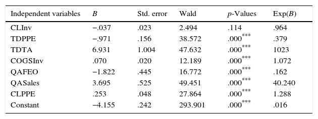
The outcomes of the classification matrix and the logistic analysis for telecommunication and information technology industry group (I4) are reported in Table 10. Financial ratios included as exogenous variables are CLInv, TDPPE, TDTA, COGSInv, QAFEO, QASales and CLPPE. The classification accuracy of the overall model is 69.7% for a 0.088 cut off score, while the classification accuracy of the non-distressed and distressed firms are 70.1% and 65% respectively – a slightly better prediction of non-distressed firms. The misclassification accuracy rate of I4 in the distressed group is the highest among all industry groups which suggests that, the model of I4 is not as powerful as other industry groups in predicting financial distress. Wald test statistics show that all of the variables, except CLInv, are statistically significant at 1% in predicting financial distress. To examine whether a reduced model better predicts financial distress, we rerun the logistic regression by dropping CLInv. However, Hosmer and Lemeshow test and Pseudo R statistics indicate that, the prediction accuracy of the actual model is greater than the reduced model. The signs of the financial ratio coefficients show that, TDPPE and QAFEO are negatively, while TDTA, COGSInv, QASales and CLPPE are positively related to financial distress. In other words, increase in financial ratios with the negative coefficients reduces the probability of financial distress, while increase in financial ratios with positive coefficients increases the probability of financial distress.
Classification matrix and logistic analysis of I4.
| Independent variables | B | Std. error | Wald | p-Values | Exp(B) |
|---|---|---|---|---|---|
| CLInv | −.037 | .023 | 2.494 | .114 | .964 |
| TDPPE | −.971 | .156 | 38.572 | .000*** | .379 |
| TDTA | 6.931 | 1.004 | 47.632 | .000*** | 1023 |
| COGSInv | .070 | .020 | 12.189 | .000*** | 1.072 |
| QAFEO | −1.822 | .445 | 16.772 | .000*** | .162 |
| QASales | 3.695 | .525 | 49.451 | .000*** | 40.240 |
| CLPPE | .253 | .048 | 27.864 | .000*** | 1.288 |
| Constant | −4.155 | .242 | 293.901 | .000*** | .016 |
| 0 | 1 | % Correctly predicted | |
|---|---|---|---|
| 0 | 1597 | 680 | 70.1 |
| 1 | 79 | 147 | 65.0 |
| Overall | 1676 | 827 | 69.7 |
This table presents the classification matrix and the logistic results of I4 industry group. Coefficients and exponential coefficients for each financial ratio are represented by B and Exp(B) respectively. Standard errors, Wald test statistics are reported along with the corresponding p-values. The cut-off score for I4 is 0.088.
The results of logistic analyses reveal that, the effect of financial ratios on the probability of financial distress varies by industry characteristics. Although an increase in a particular ratio may increase the likelihood of financial distress for a certain industry group, it may actually reduce it for another. For instance, CashTA and CashTL ratios have the opposite signs in I2 and I3 industry groups. Similarly, the sign of the SalesPPE ratio is negative in I1 and I3, while it is positive in I2 industry group. Moreover, COGSInv and InvSales ratios are negatively related to financial distress in I1, while they are positively related in I2 and I3 industry groups. Thus, it is clear that there are industry related factors influencing distress probability and hence industry specific models tend to do better than a single, general distress prediction model.
Finally, we present below the industry specific FD models for I1, I2, I3 and I4 industry groups from the logistic regression. The estimated logistic regression model for group I1 is:
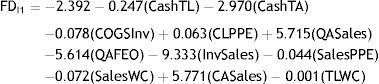
FDI1 model misclassifies 663 out of 4011 cases (cases with missing data are excluded) achieving a classification accuracy of 83.5%.7 For the I2 group we estimate the following logistic regression model:
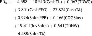
FDI2 model misclassifies only 88 out of 838 of the cases, achieving an accuracy of 89.5%. The estimated logistic regression model for financial distress for industry group I3 is:
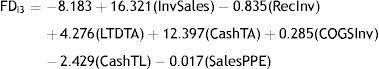
Model FDI3 misclassifies only 135 out of 4300 of the cases for a classification accuracy rate of 96.9%. Finally, for I4 group, the estimated FD model is:
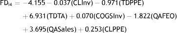
Model FDI4 misclassifies 228 out of 25,103 for a classification accuracy rate of 90.9%. In summary, we can state that the industry specific financial distress models accurately predict financial distress.
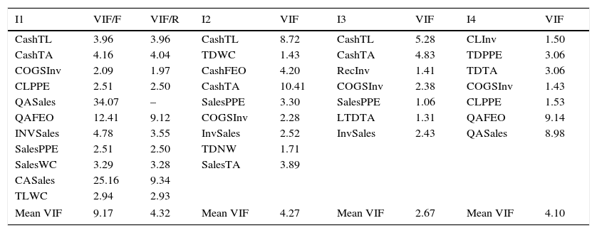
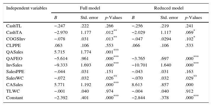
Robustness testsThe central idea for factor analysis is to minimize a dataset which may include a large number of interrelated variables, while retaining as much of the variation in the dataset (Jolliffe, 2002). As is generally done in the literature, this study employed factor analysis to prevent information redundancy by limiting the level of multicollinearity among the financial ratios (Laurent, 1979). As a second check to avoid possible overlaps between the ratios, we also run multicollinearity tests for the financial ratio sets of each industry group. As a rule of thumb, variance inflation factor (VIF) greater than 10 may indicate multicollinearity and it requires further investigation. Table 11 shows that VIF scores of the financial rations in I2, I3 and I4 industry groups do not exceed the critical value. However, in I1 industry group, three ratios have VIF scores that exceed ten. To investigate this further, we omit – QASales – which has the highest VIF score in the logistic model for I1. Table 12 shows that, despite the level of significance for CashTA and COGSInv decline from 5% to 10%, the sign of the coefficients do not change and variables which are significant in the full model remain significant in the reduced model. Moreover, the coefficient standard errors, both in the full and the reduced models are not inflated suggesting that the coefficient estimates are robust in the full model (Gunst, 1983; Lennox et al., 2012). In the end, comparison of the reduced and the full models indicate that the model with all the financial ratios is legitimate as multicollinearity is not a serious problem and the coefficient estimates do not include any significant bias.
Multicollinearity test.
| I1 | VIF/F | VIF/R | I2 | VIF | I3 | VIF | I4 | VIF |
|---|---|---|---|---|---|---|---|---|
| CashTL | 3.96 | 3.96 | CashTL | 8.72 | CashTL | 5.28 | CLInv | 1.50 |
| CashTA | 4.16 | 4.04 | TDWC | 1.43 | CashTA | 4.83 | TDPPE | 3.06 |
| COGSInv | 2.09 | 1.97 | CashFEO | 4.20 | RecInv | 1.41 | TDTA | 3.06 |
| CLPPE | 2.51 | 2.50 | CashTA | 10.41 | COGSInv | 2.38 | COGSInv | 1.43 |
| QASales | 34.07 | – | SalesPPE | 3.30 | SalesPPE | 1.06 | CLPPE | 1.53 |
| QAFEO | 12.41 | 9.12 | COGSInv | 2.28 | LTDTA | 1.31 | QAFEO | 9.14 |
| INVSales | 4.78 | 3.55 | InvSales | 2.52 | InvSales | 2.43 | QASales | 8.98 |
| SalesPPE | 2.51 | 2.50 | TDNW | 1.71 | ||||
| SalesWC | 3.29 | 3.28 | SalesTA | 3.89 | ||||
| CASales | 25.16 | 9.34 | ||||||
| TLWC | 2.94 | 2.93 | ||||||
| Mean VIF | 9.17 | 4.32 | Mean VIF | 4.27 | Mean VIF | 2.67 | Mean VIF | 4.10 |
This table shows the variance inflation factor (VIF) scores for I1, I2, I3 and I4 industry groups respectively. Particularly for the I1 industry group VIF/F presents the VIF scores for the full sample and VIF/R for the restricted sample when QASales is omitted. I1 includes firms in the consumer staples, consumer discretionary and health care industries, I2 includes firms in the energy and utility industries, I3 presents firms in the industrials and basic materials and I4 comprises of firms in the telecommunication services and information technology industries.
Multicollinearity test – comparison of the full and the reduced models of I1.
| Independent variables | Full model | Reduced model | ||||
|---|---|---|---|---|---|---|
| B | Std. error | p-Values | B | Std. error | p-Values | |
| CashTL | −.247 | .222 | .266 | −.256 | .219 | .241 |
| CashTA | −2.970 | 1.177 | .012** | −2.029 | 1.117 | .069* |
| COGSInv | −.078 | .031 | .013** | −.047 | .0294 | .102* |
| CLPPE | .063 | .106 | .553 | .066 | .106 | .533 |
| QASales | 5.715 | 1.774 | .001*** | |||
| QAFEO | −5.614 | .961 | .000*** | −3.765 | .697 | .000*** |
| InvSales | −9.333 | 1.693 | .000*** | −10.701 | 1.640 | .000*** |
| SalesPPE | −.044 | .031 | .151 | −.043 | .031 | .163 |
| SalesWC | −.072 | .032 | .026** | −.070 | .032 | .029** |
| CASales | 5.771 | 1.192 | .000*** | 8.613 | .857 | .000 |
| TLWC | −.001 | .040 | .974 | −.004 | .040 | .912 |
| Constant | −2.392 | .401 | .000*** | −2.844 | .378 | .000*** |
This table presents the comparison of the logistic regression analysis of I1 industry group between the full and the restricted model when QASales is omitted. I1 includes firms in the consumer staples, consumer discretionary and health care industries.
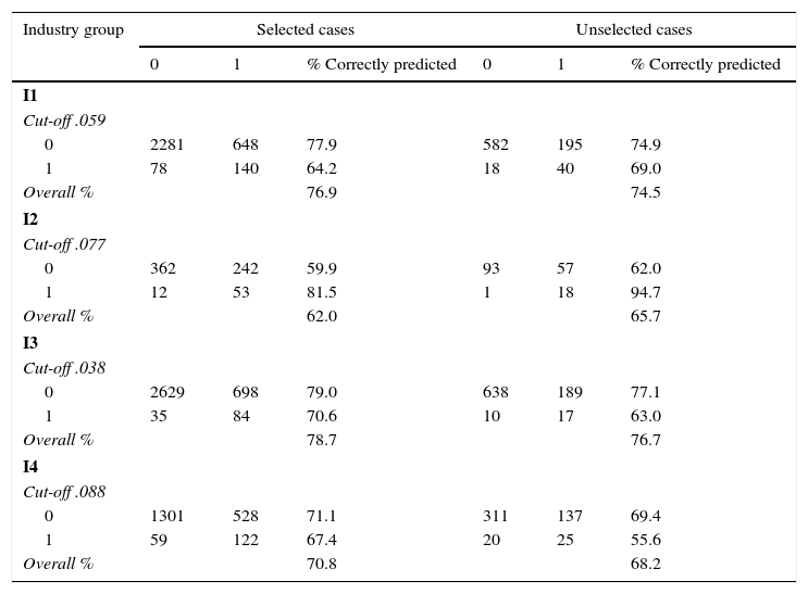
To examine whether prediction accuracy of the financial distress model developed by the logistic analysis holds also for a restricted sample, we conduct split-sample validation test for each industry group. For this purpose, we performed 80–20 split-sample validation, where 80% of the sample data is randomly selected as the training sample and 20% as the hold out sample.8 In order to make sure that the accuracy of the financial distress models hold for the restricted sample of data we check for two issues. First, we check whether the difference of total accuracy rates between the training and the hold out sample exceeds 10%. Second, we examine whether the overall accuracy rate is greater than 50% for both the training and the hold out sample. If the difference of the accuracy rates between the samples exceeds 10%, it would indicate that the prediction accuracy of the model varies between subsamples (James et al., 2005). Additionally, if the overall accuracy rate is below 50%, we can state that the model predicts financial distress not any better than predicting by chance (Hair et al., 2005).
Table 13 shows the classification accuracy table of the validation sample for each industry group. The results for the I1 group reveal that, overall classification accuracy of the training sample is 76.9% and for the holdout sample it is 74.5%. Likewise, the accuracy rates for I2 are 63% and 65.7%, for I3 they are 78.7% and 76 and for I4 they are 70.8% and 68.2% respectively for training and hold out samples. In all cases the 10% criterion is satisfied lending further support to the accuracy of the industry-specific financial distress prediction models.
Classification matrix of the validation sample.
| Industry group | Selected cases | Unselected cases | ||||
|---|---|---|---|---|---|---|
| 0 | 1 | % Correctly predicted | 0 | 1 | % Correctly predicted | |
| I1 | ||||||
| Cut-off .059 | ||||||
| 0 | 2281 | 648 | 77.9 | 582 | 195 | 74.9 |
| 1 | 78 | 140 | 64.2 | 18 | 40 | 69.0 |
| Overall % | 76.9 | 74.5 | ||||
| I2 | ||||||
| Cut-off .077 | ||||||
| 0 | 362 | 242 | 59.9 | 93 | 57 | 62.0 |
| 1 | 12 | 53 | 81.5 | 1 | 18 | 94.7 |
| Overall % | 62.0 | 65.7 | ||||
| I3 | ||||||
| Cut-off .038 | ||||||
| 0 | 2629 | 698 | 79.0 | 638 | 189 | 77.1 |
| 1 | 35 | 84 | 70.6 | 10 | 17 | 63.0 |
| Overall % | 78.7 | 76.7 | ||||
| I4 | ||||||
| Cut-off .088 | ||||||
| 0 | 1301 | 528 | 71.1 | 311 | 137 | 69.4 |
| 1 | 59 | 122 | 67.4 | 20 | 25 | 55.6 |
| Overall % | 70.8 | 68.2 | ||||
This table shows the 80–20 split-sample validation test results for the I1, I2, I3 and I4 industry groups where randomly selected 80% of the sample are classified in the training sample and 20% are classified in the hold-out sample. I1 includes firms in the consumer staples, consumer discretionary and health care industries, I2 includes firms in the energy and utility industries, I3 presents firms in the industrials and basic materials and I4 comprises of firms in the telecommunication services and information technology industries.
This study attempts to formulate industry specific financial distress models to reduce the information mass available to financial statements users. For this purpose, we first employ a factor analysis to derive the most informative financial ratios showing stable patterns over the period 1990–2011 for each industry group. After obtaining the initial ratio set for each industry group, we conduct entropy method to single out financial ratios that possess the highest information content in determining uncertainty levels for each industry group. In line with the literature, the outcomes show that liquidity ratios (i.e. CashTA, CashTL and CashFEO) have the highest information content in majority of the industries (Casey and Bartczak, 1985; Stanca and Gallegati, 1999) as the disclosure of these items provide more timely information as well as information about uncertainty of firms for financial statement users. Moreover, the results also show that the information content of the inventory intensive and solvency ratios diverge among the industry groups. For instance, inventory intensive ratios (i.e. COGSInv and RecInv) are more informative in consumer staples, consumer discretionary, health, industrials and basic materials, while solvency ratios (i.e. TDWC, TDPPE, TDTA and CLInv) have greater information content in energy, utility, telecommunications and information technology industries (Cambini and Rondi, 2012). The reason for these differences between the industry groups may lie in the fact that the I2 and I4 groups necessitate huge amounts of financial support in order to stay competitive in the market. These technology intensive industries should maintain competitive advantage and fight against “bigger and better” responses from competitors in the form of newly developed technologies (Afuah and Utterback, 1997). Hence, to preserve competitive advantage, technology intensive firms have to initiate their business to leverage newly found products (Kettinger et al., 1994). In this regard, it is not surprising that, information content of financial leverage ratios is greater than those related to liquidity.
We use industry specific financial ratios derived from the entropy method as independent variables in the logistic regression analysis and attempt to build industry specific financial distress models. The results show that, industry specific financial distress models for all of the industry groups accurately predict financial distress, while classification accuracy rates diverge between the industry groups.
These models show that, the effect of financial ratios on the probability of financial distress varies across industries. For instance, there are cases where the same predictor variable (ratio) has different coefficient signs in different industry groups which may be due to several factors. Industry characteristics might be one reason for diverging impact of financial ratios on firms’ distress. For instance, inventory types of the energy and utility industries are completely different from manufacturing industry, since most of the inventories of energy and utility industries consist of spare parts, while the inventories of manufacturing industry also include raw materials, work in process and finished goods. Similarly, the inventory behavior of durable and non-durable goods also varies in terms of length of production and stock turnover period, output-stock equilibrium level, volume of production of purchased materials, goods in process and finished goods as well as sales volume and expectations (Lovell, 1961). Likewise, fixed asset composition (plant size, level of mechanization, vertical integration, nature of the production process and etc.) and sales behavior are also completely different between the utility and manufacturing industries. In order to examine the relation of SalesPPE ratio to financial distress in these industry groups, we should consider production characteristics of the industries, such as capacity utilization, structure of the assets (whether they are owned or leased for a certain period), age of the plants and managerial efficiency. We should also consider economic characteristics of the industries, since they directly affect the level of fixed asset turnover. To give an example, industries that produce apparel, leather, tobacco, furniture and food tend to have greater fixed asset turnover than other industries, since their asset structure are directly related to their manufacturing operations. On the contrary industries such as primary metal and petroleum possess lower levels of fixed assets since they hold higher volumes of natural resources, which are only indirectly related to manufacturing operations (Gupta and Huefner, 1972). Hence, the sign of the ratios would likely to differ between industry groups as a result of varying industry and economic characteristics.
Additionally, the sign of the coefficients for the same predictor variables might vary between industry groups since the optimum level for each financial ratio differs not only by industry group but also by firm depended on the firm structure. Since the effect of financial ratios on the financial distress of firms is parabolic, it is possible for a financial ratio to reduce the financial distress as it increases up to an optimum level and increase the probability past the optimum. To give an example, increase in the level of CashTA can be interpreted as a sign of short term liquidity, since high levels of cash holdings would likely to reduce transaction costs and serves as a buffer in meeting highly volatile input prices (Baum et al., 2006). On the other hand, after a certain level of liquidity, further increases in cash holdings can be a sign of a slowdown in the evaluation process of long term investment opportunities. Because firms’ liquidity decisions are taken by management based on future profit expectations, capital investment needs and the uncertainty level of the firms’ industry, an increase in the CashTA ratio up to a certain level can be a sign of financial health, while after that level, its positive effect on financial health would likely to disappear. Such scenarios can be extended for all the financial ratios that provide information about the optimum asset and capital structure of a firm. For that reason, we can state that, since financial ratios are nonlinearly related to financial distress variable, sign of the coefficients of predictor variables would likely to vary between industry groups.
In general, the results demonstrate the importance of using industry specific financial ratios in determining the level of financial distress. Since the industry specific financial distress models provide detailed information about industry specific risks along with industry characteristics, financial statement users would benefit from employing them in decision making.
Our results could have several direct applications. First, it identifies those financial ratios which are most appropriate and important for a particular industry. Since industry characteristics are very difficult to be enumerated and quantified individually, it is important to observe the financial ratios that incorporate a certain set of industry characteristics. Second, since there are a large number of financial ratios, financial statement users face the problem of selecting relevant information. Thus, our results would contribute to the literature by providing an optimal set of ratios. Moreover, this study also provides useful insights to the financial statement users in assessing the financial distress of firms. Although there are numerous financial distress models in the accounting literature, they lack industry related information and treat all firms equally, even though they are from different industries. Since we use industry specific financial ratios in constructing separate financial distress models for each industry group, prediction accuracy of our models benefit from the industry related information as well. As a consequence, industry specific financial distress models would find applicability in notifying financial statement users regarding the reasons of financial distress for different industry groups.
For future research, industry specific financial ratios can be analyzed in detail, and the mean values of distressed firms’ financial ratios for each industry group could be compared to the actual industry averages to see whether firms classified as distressed by the industry specific FD models possess financial ratio levels below industry averages. In building financial distress models, this study does not use matched sample design and does not determine a range for mean asset size of distressed and non-distressed firms. Consequently, as a future research subject, distressed and non-distressed firms could be matched in terms of asset size to evaluate whether an improvement in the prediction accuracy rate of FD models would be observed. Finally, industry specific FD model can be applied to a broader data set including all publicly traded US firms to test the generalizability of the outcomes.
The authors would like to thank Umit Akinc (Professor at WFU) and Carol Cain (Professor at WFU) for providing language help and writing assistance. This work was supported by the Scientific and Technological Research Council of Turkey (TUBITAK) under grant no: B.14.2.TBT.0.06.01-219-115543.
Earnings Before Interest and Taxes/Total Assets (EBITTA), Net Income/Total Assets (NITA), Funds Flow from Operations/Total Assets (FFOTA), Net Income/Total Liabilities (NITL), Funds Flow from Operations/Total Liabilities (FFOTL), Net Income/Net Worth (NINW), Funds Flow from Operations/Net Worth (FFONW), Earnings Before Interest and Taxes/Net Sales (EBITSales), Long Term Debt/Total Assets (LTDTA), Long Term Debt/Total Liabilities (LTDTL), Total Assets/Net Worth (TANW), Total Liabilities/Total Assets (TLTA), Total Debt/Property, Plant and Equipment (TDPPE), Total Liabilities/Net Worth (TLNW), Total Debt/Net Worth (TDNW), Total Debt/Total Assets (TDTA), Funds Flow from Operations/Total Debt (FFOTD), Total Debt/Working Capital (TDWC), Total Liabilities/Working Capital (TLWC), Funds Flow from Operations/Working Capital (FFOWC), Net Income/Working Capital (NIWC), Inventory/Working Capital (InvWC), Current Assets/Total Assets (CATA), Funds Flow from Operations/Net Sales (FFOSales), Net Income/Net Sales (NISales), Current Liabilities/Property, Plant and Equipment (CLPPE), Quick Assets/Total Assets (QATA), Net Worth/Net Sales (NWSales), Net Sales/Total Assets (SalesTA), Net Sales/Property, Plant and Equipment (SalesPPE), Inventory/Net Sales (InvSales), Current Liabilities/Inventory (CLInv), Working Capital/Total Assets (WCTA), Current Assets/Net Sales (CASales), Net Sales/Working Capital (SalesWC), Cost of Goods Sold/Inventory (COGSInv), Earnings Before Interest and Taxes/Interest Expense (EBITIntExp), Current Assets/Net Worth (CANW), Dividend/Net Income (DivNI), Current Assets/Current Liabilities (CACL), Quick Assets/Current Liabilities (QACL), Cash and Cash Equivalents/Total Assets (CashTA), Cash and Cash Equivalents/Total Liabilities (CashTL), Quick Assets/Funds Expenditures for Operations (QAFEO), Cash and Cash Equivalents/Funds Expenditures for Operations (CashFEO), Net Receivables/Inventory (RecInv), Inventory/Current Assets (InvCA), Receivables/Net Sales (RecSales), Quick Assets/Net Sales (QASales), Quick Assets/Cash Flow from Operations (QACFO), Current Assets/Cash Flow from Operations (CACFO).
| Industry group | −2 log likelihood | Omnibus test | Pseudo R statistics | Hosmer and Lemeshow test | ||||||
|---|---|---|---|---|---|---|---|---|---|---|
| χ2 | df | p-Value | Cox–Snell R2 | Nagelkerke R2 | χ2 | df | p-Value | |||
| I1 | Step 0 | 2005.8 | 332.1 | 11 | .000*** | .080 | .202 | 12.22 | 8 | .141 |
| Step 1 | 1673.7 | |||||||||
| I2 | Step 0 | 545.7 | 72.19 | 9 | .000*** | .083 | .172 | 12.93 | 8 | .114 |
| Step 1 | 473.5 | |||||||||
| I3 | Step 0 | 1274.8 | 246.9 | 7 | .000*** | .056 | .218 | 11.41 | 8 | .179 |
| Step 1 | 1027.8 | |||||||||
| I4 | Step 0 | 1517.8 | 135.1 | 7 | .000*** | .053 | .116 | 12.49 | 8 | .131 |
| Step 1 | 1382.7 | |||||||||
This table shows the goodness of fit model including Omnibus test statistics, Pseudo R statistics and Hosmer and Lemeshow test statistics for the industry groups I1, I2, I3 and I4.
Significance at .01 level.
I1 includes firms in the consumer staples, consumer discretionary and health care industries, I2 includes firms in the energy and utility industries, I3 presents firms in the industrials and basic materials and I4 comprises of firms in the telecommunication services and information technology industries.
Before starting the analysis, we check whether our data satisfies the necessary assumptions of factor analysis. Contrary to other multivariate techniques, assumptions of factor analysis are more conceptual than statistical. In other words, rather than emphasizing the statistical qualities of variables included, factor analysis centers its concerns on the character and composition of variables. In practical terms, factor analysis assumes normality, homoscedasticity and linearity. To handle variables with high standard deviations and to avoid cases with extreme outliers, we use an outlier cut off value of 4 standard deviations and delete those cases which exceed that cut off point. As a result of this data quality improvement process, even though Kolmogorov–Smirnov test does not support normality assumption, Stem&Leaf plots, P–P plots and histogram analysis show that financial ratios demonstrate normal distributions around the mean with tolerable standard deviations. The intercorrelation matrices among the financial ratios show sufficient correlation levels to justify factor analysis.
Tables that show factor loadings of financial ratios including the periods 1990–2000 and 2001–2011 for each industry group can be provided by the authors upon request.
Entropy scores for the entire financial ratio set can be provided by the authors upon request.
In the model type I error corresponds to the number of non-distressed firms classified as distressed; and type II error vice versa.
Iteration history of the industry groups can be provided by the authors upon request.
Wald test statistics for a particular variable indicate the extent of the effect of the variable on the estimated probability and prediction of group membership.
Detailed results will be provided by the authors upon request.
We employed “Uniform” function to generate random values in SPSS, where the minimum value is set to 0 and maximum value is set to 1. The random values generated which are less than 0.80 are classified in the training sample and the rest is classified in the hold out sample.