A geostatistical re-interpretation of gravity surveys in the Yagoua, Cameroon region

Resumen

Desde 1960 se han realizado diversos estudios de gravedad en la región Yagoua del norte de Camerún. Se recabaron datos de gravedad en una área amplia que abarca aproximadamente 11.628 km². Estos datos son insuficientes, irregulares, dispersos y no permiten eficientemente continuaciones ascendentes y descendentes del campo gravitatorio, derivadas y otras operaciones que requieren datos reticulados regulares. Algunas anomalías en el mapa Collignon (1968) pueden correlacionarse con la estructura geológica que se conoce, pero no aparecen en los mapas de Louis (1970) y Poudjom et al. (1996). Para producir los datos de gravedad reticulares regulares y mejor control de las anomalías, derivadas de estructuras geológicas, se aplicó el método de Kriging a una línea de base de datos-188. Se ensayaron para este propósito varios modelos de variograma. Se encontró que un modelo esférico era la mejor opción; se ha elaborado un nuevo conjunto de datos Kriging con unos 10.100 resultados y un nuevo mapa con los datos Kriged Bouguer. Este mapa contiene anomalías positivas en las zonas Maroua-Mindif y Maga (1968) en el mapa Collignon, que no estaban presentes en los mapas de Louis (1970) y Poudjom et al. (1996). Las anomalías positivas de Guibi-Doukoula y Yagoua, que no se encuentran separados en los mapas de Louis (1970) y Poudjom et al. (1996), aparecen claramente distintas a como fueron previstas por Collignon (1968). Los nuevos resultados pueden ser utilizados para los estudios gravimétricos posteriores.

Abstract

Since 1960, many gravity studies have been carried out in the Yagoua region of northern Cameroon. Gravity data was collected over a wide area of approximately 11628 km². These data are insufficient, irregular, scattered and do not efficiently permit gravity field downward and upward continuations, derivatives and other operations that might require regular gridded data. Some anomalies on the Collignon map (1968), may correlate with known geological structure but do not appear on maps by Louis (1970) and Poudjom et al. (1996). To produce regular gridded gravity data and better control anomalies due to geological structures, the kriging method was applied to a 188-data baseline. Several variogram models were tested for this purpose. It was found that a spherical variogram model is the best; it has produced a new kriging dataset of about 10,100 data and a new map of kriged Bouguer data. This map contains positive anomalies in the Maroua-Mindif and Maga areas on the Collignon (1968) map, which were not present on Louis (1970) and Poudjom et al. (1996) maps. The positive anomalies of Guibi-Doukoula and Yagoua, not separated on the Louis (1970) and Poudjom et al. (1996) maps, show up as clearly distinct as previewed by Collignon (1968). The new results can be used for subsequent gravimetric studies.

Introduction

Geostatistics is applied in the Earth sciences as an interpolation procedure that uses an available dataset to obtain an optimal, linear and unbiased estimation of a property whose estimation error is minimized (Matheron, 1973). It operates on a random variable for which a set of possible values is known but whose final result requires a measurement. The objective of this study is to re-examine a gravity data set from irregular gridded data. For this operation known as kriging, we make a crucial choice of a variogram. This is a better choice, because more kriged values are closer to reality. The principal difficulty is to find a variogram model that fits the data to be interpolated. In this work, we calculate an experimental variogram from existing gravity data, we evaluate the RMS between the variogram and we use various cross-data validation criteria to ensure that the variogram model chosen is optimal in order to correlate with the experimental variogram. We also offer a new gravity dataset and we propose a new gravity map of the Yagoua region in northern Cameroon.

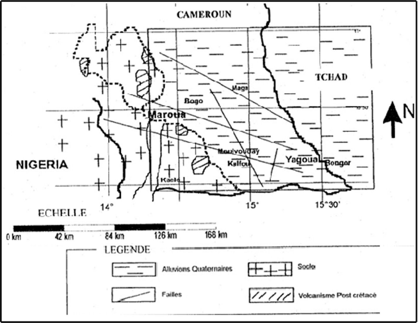
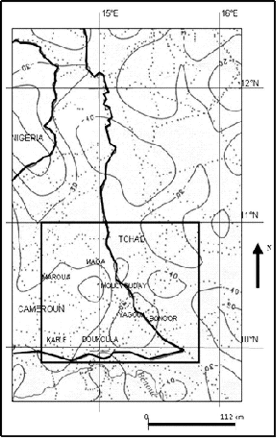
Study area and Gravity data

Presentation of the study area

Yagoua region (Figure 1), as others in Central-Africa, is the product of a complex period of continental disruption associated to plate tectonic fragmentation of Gondwana (Genik, 1992; Njandjock, 2004). It is characterised by polyphase rifting, separated by tectonic events that can be linked to regional deformation, hiatus of sedimentation and unconformities in seismic sections and outcrops. The region belonging to the Panafrican belt, is bounded to the South by the Doba basin, to the North by Lake Chad basin, to the East by Doseo and Salamat basins, and to the North West by the Mandara Mountains and the Southeast by the Kaele dome. The study area in Cameroon, covers an area of about 11628 km² and stretches from latitude 9°45 ‘N to 10°47’N to longitude 14°20’ E to 15°30’E.

Figure 1.

Simplied geology map of the study area.

Geological context

The Yagoua region is located in the southern part of the Logone Birni Basin (LBB) characterised by Quaternary sediments and belonging to the West and Central African Rift System. The geology of the region (Figure 1) is underlain by a large sedimentary formation and a Precambrian basement. The basement consists of acid and metamorphic formations. gneisses, migmatites, diorites, anatexites, syenites, syn-tectonic to post-tectonic granites, basalts and shales. Rare basalts are observed in the Kaélé region (Maurin, 2002). Among the bedrock outcrops, the Precambrian is dominant. It is characterized by migmatites and anatexites located southwest of the region in Maroua and Kaélé. Some remarkable features include the Mindif intrusion composed of syenites (Eno Belinga, 1984), the North Maroua gabbro hills and the Kaélé hills. The sedimentation in this area commenced during the Neocomian-Albian rifting period and consists of sandstones, clays and shales. The sedimentary formation is everywhere overlain by sandy alluvial formations and dunes attributable to the Pre-Bima formation (Louis, 1970; Genik, 1992).

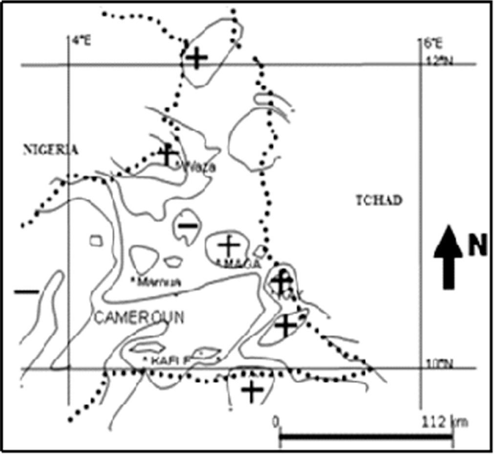
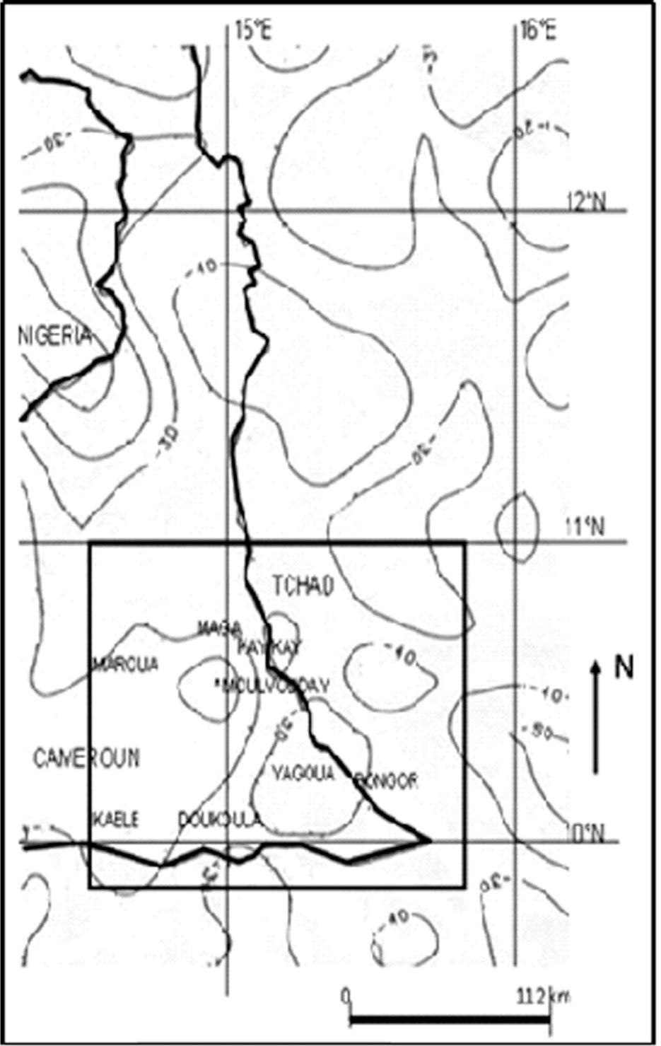
Gravity data

Gravity data used in this study were acquired during surveys conducted by various organizations and researchers: Collignon (1968); Louis (1970); Elf-Serepca, 1980; Poudjoum et al., 1995-1996; Njandjock, 2002 to 2004 and Njandjock et al., 2006. Measurements were carried out along profiles to detect significant variations of geological facies. The station locations were obtained from topographic maps and compass traverses. The elevation of the stations was obtained from barometric readings, using Wallace and Tierman or Thomnen altimeters. Variations in the gravity field were measured using Worden, Lacoste & Romberg and North American gravimeters. The gravity data were converted to Cartesian coordinates and need to be interpolated. The conversion to kilometric distances was by UTM (Universal Transverse Mercator) on the Clarke’s ellipsoid (1880) with the Prime Meridian. Bouguer anomaly maps by Collignon(1968), Louis (1970) and Poudjom (1996) are shwon on Figures 2, 3, 4 and 5.

Figure 2.

Bouguer anomaly map of Yagoua region (Collignon, 1968).

Figure 3.

Bouguer anomaly map of Yagoua region. (Louis, 1970).

Figure 4.

Bouguer anomaly map of Yagoua region. (Poudjom, 1996).

Figure 5.

Distribution of gravity data in the study area.

Method

The main purpose of a geostatistical study is to construct a mathematical model of the random function Z (X), based on an experimental data set Z_exp (X_i), a single realization of Z (X), where x and x + h are two points separated by a distance h, and z (x) and z(x + h) are associated random variables. The variogram is known and the semi-variance of the difference [z (x)-z (x + h)] is (Chiles and Delfiner, 1999; Kumar and Remadevi 2006):

Experimentally, it is calculated by the equation

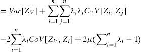
Supposing that we want to estimate a block V centered at X₀. Z_V denote the true value (unknown) of this block and Z_V^* the estimate that is obtained:

Z_i being the random variables corresponding to sample points. We want to minimize

Substituting the expression of the estimated in this equation, we obtained

Since the estimate is unbiased, we set

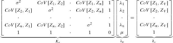
To minimize σe2, we use Lagrange’s method and we form the Lagrangian

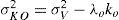
Where μ is the Lagrange multiplier. The minimum is reached when all the λ_i and μ partial derivatives are canceled out. This leads to the following ordinary kriging system:

Minimum variance estimation called kriging variance is obtained by substituting the kriging equations in the general expression of the variance estimation.

In the matrix form, these equations are written as

Results and Discussion

Experimental variogram of the Yagoua region

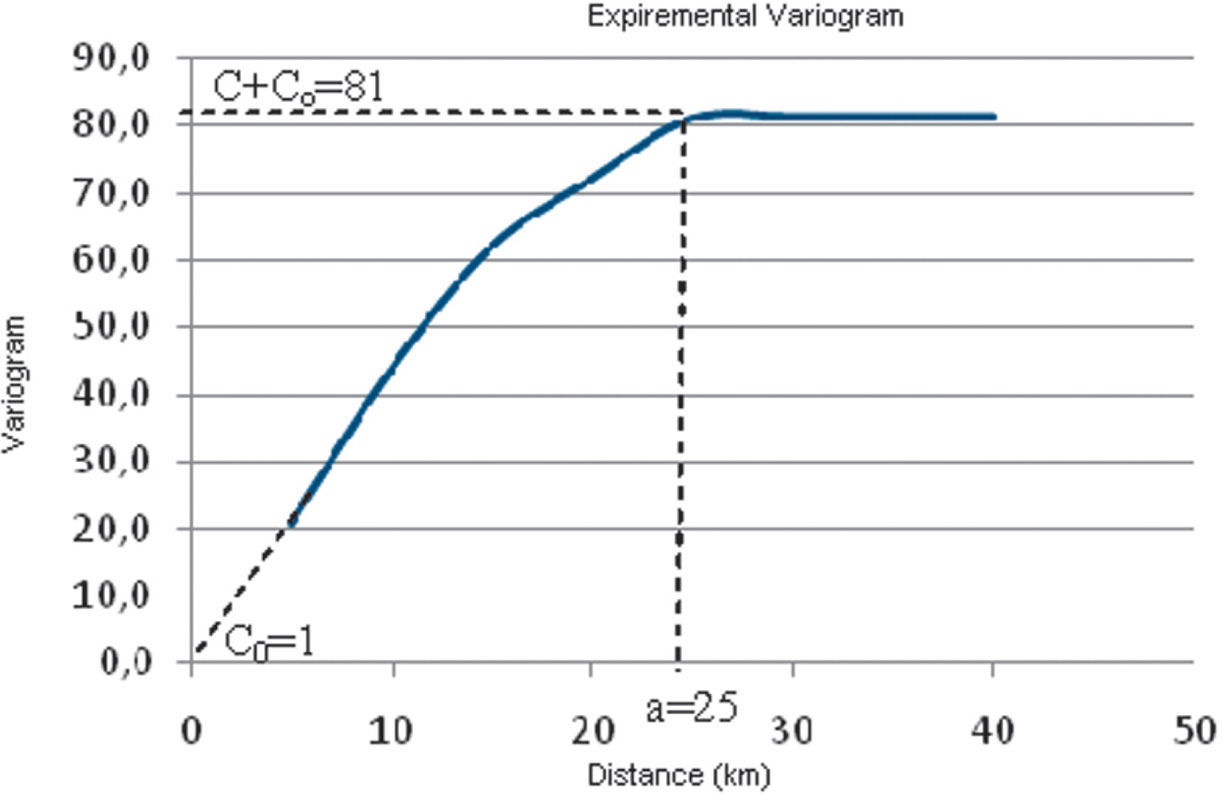
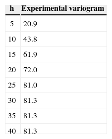
The experimental variogram is now calculated from equation (2). Results are ranked by increasing distance, and then grouped in intervals centered on increasing multiples of h= 5. The results shown in Table 1, are used to plot the variogram (Figure 6).

Table 1.

Experimental variogram values of Bouguer anomalies corresponding to the pitch h.

h	Experimental variogram
5	20.9
10	43.8
15	61.9
20	72.0
25	81.0
30	81.3
35	81.3
40	81.3

Figure 6.

Experimental variogram of gravity data from the Yagoua region.

The variogram characteristics are: range a = 25; level C + C₀ = 81; nugget; C₀ = 1.

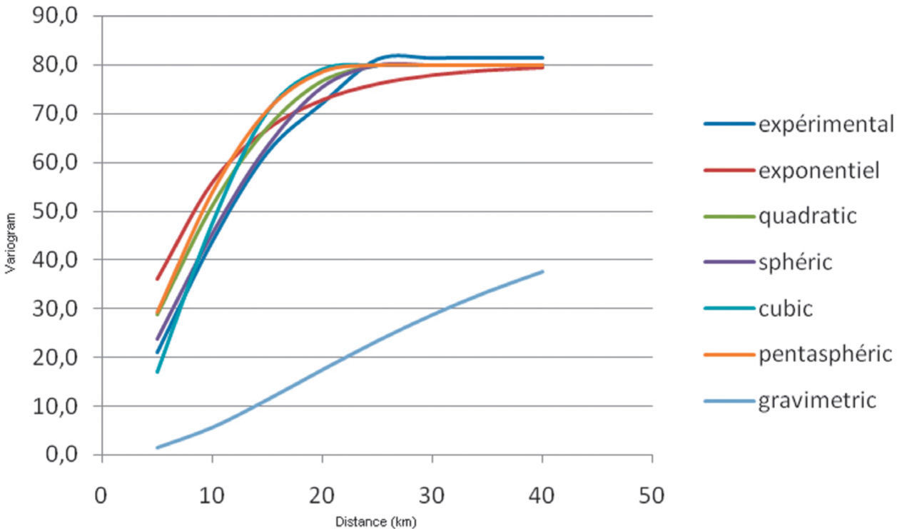
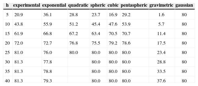
The known mathematical variogram models in the literature were used to calculate different models of variograms and compare them to the experimental one (Figures 6 and7). The results are summarized in Table 2. In these calculations, several models (for example the Gaussian model) not shown here have been eliminated. The superposition of curves giving the variogram as a function of h is given in Figure 7. The dark blue curve represents the experimental variogram of the Yagoua region. Our aim is to find among the other curves of this graph the one that best approximates the dark blue curve. The outer gray curve represents the gravity model whose elimination is visible; it is difficult to comment on the other curves. Indeed within this paragraph, it is difficult to say exactly which curve (red, green, purple, blue or orange) is closest to the dark blue curve. Qualitatively all these models are eligible. For this reason we will make a quantitative analysis using the equation

Figure 7.

Superposition of the curves giving the variogram according to the pitch h.

Table 2.

Variograms of different models and compare the experimental variogram.

h	experimental	exponential	quadratic	spheric	cubic	pentaspheric	gravimetric	gaussian
5	20.9	36.1	28.8	23.7	16.9	29.2	1.6	80
10	43.8	55.9	51.2	45.4	47.6	53.9	5.7	80
15	61.9	66.8	67.2	63.4	70.5	70.7	11.4	80
20	72.0	72.7	76.8	75.5	79.2	78.6	17.5	80
25	81.0	76.0	80.0	80.0	80.0	80.0	23.4	80
30	81.3	77.8		80.0	80.0	80.0	28.8	80
35	81.3	78.8		80.0	80.0	80.0	33.5	80
40	81.3	79.3		80.0	80.0	80.0	37.6	80

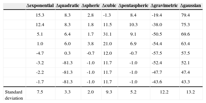
to calculate the relative changes, and standard deviation of these relative changes between each variogram model and the experimental variogram.

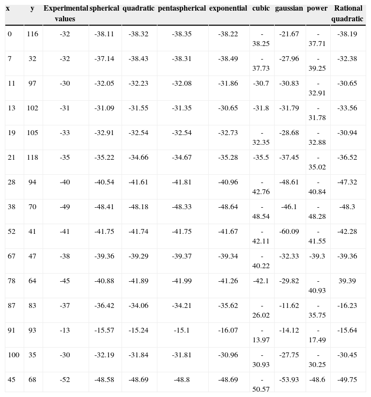
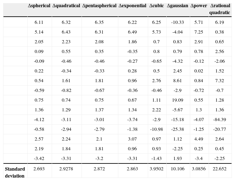
Changes between experimental variogram values and those of different models are reported in Table 3. The standard deviation values between the experimental variogram and the different model is 2.0 for spherical, 3.3 for quadratic, 5.2 for pentaspherical, 7.5 for exponential and 13.2 for Gaussian (Table 3). It is clear that the model giving the best variogram model are the spherical, tracking quadratic and pentaspherical models. In order to confirm or invalidate this result, we made kriged maps using several models. The goal is to determine which variogram model reproduces the experimental values. For this purpose, we have omitted 15 of the 188 baseline. Then we realized the kriged map of spherical, square, pentaspherical, exponential, cubic, Gaussian, rational quadratic and power models with the 173 remaining data. On these kriged maps, we reported values of anomalies the hidden points. Abnormal values obtained by kriging with different variogram models are shown in Table 4. The relative differences between the anomalies from various models and the current anomalies are contained in table 5.

Table 3.

First standard derivation of different models.

	Δexponential	Δquadratic	Δspheric	Δcubic	Δpentaspheric	Δgravimetric	Δgaussian
	15.3	8.3	2.8	-1.3	8.4	-19.4	79.4
	12.4	8.3	1.8	11.5	10.3	-38.0	75.3
	5.1	6.4	1.7	31.1	9.1	-50.5	69.6
	1.0	6.0	3.8	21.0	6.9	-54.4	63.4
	-4.7	0.3	-0.7	12.0	-0.7	-57.5	57.5
	-3.2	-81.3	-1.0	11.7	-1.0	-52.4	52.1
	-2.2	-81.3	-1.0	11.7	-1.0	-47.7	47.4
	-1.7	-81.3	-1.0	11.7	-1.0	-43.6	43.3
Standard deviation	7.5	3.3	2.0	9.3	5.2	12.2	13.2

Table 4.

Variograms of different models and the experimental values.

x	y	Experimental values	spherical	quadratic	pentaspherical	exponential	cubic	gaussian	power	Rational quadratic
0	116	-32	-38.11	-38.32	-38.35	-38.22	-38.25	-21.67	-37.71	-38.19
7	32	-32	-37.14	-38.43	-38.31	-38.49	-37.73	-27.96	-39.25	-32.38
11	97	-30	-32.05	-32.23	-32.08	-31.86	-30.7	-30.83	-32.91	-30.65
13	102	-31	-31.09	-31.55	-31.35	-30.65	-31.8	-31.79	-31.78	-33.56
19	105	-33	-32.91	-32.54	-32.54	-32.73	-32.35	-28.68	-32.88	-30.94
21	118	-35	-35.22	-34.66	-34.67	-35.28	-35.5	-37.45	-35.02	-36.52
28	94	-40	-40.54	-41.61	-41.81	-40.96	-42.76	-48.61	-40.84	-47.32
38	70	-49	-48.41	-48.18	-48.33	-48.64	-48.54	-46.1	-48.28	-48.3
52	41	-41	-41.75	-41.74	-41.75	-41.67	-42.11	-60.09	-41.55	-42.28
67	47	-38	-39.36	-39.29	-39.37	-39.34	-40.22	-32.33	-39.3	-39.36
78	64	-45	-40.88	-41.89	-41.99	-41.26	-42.1	-29.82	-40.93	39.39
87	83	-37	-36.42	-34.06	-34.21	-35.62	-26.02	-11.62	-35.75	-16.23
91	93	-13	-15.57	-15.24	-15.1	-16.07	-13.97	-14.12	-17.49	-15.64
100	35	-30	-32.19	-31.84	-31.81	-30.96	-30.93	-27.75	-30.25	-30.45
45	68	-52	-48.58	-48.69	-48.8	-48.69	-50.57	-53.93	-48.6	-49.75

Table 5.

Second standard derivation of different models.

	Δspherical	Δquadratical	Δpentaspherical	Δexponential	Δcubic	Δgaussian	Δpower	Δrational quadratic
	6.11	6.32	6.35	6.22	6.25	-10.33	5.71	6.19
	5.14	6.43	6.31	6.49	5.73	-4.04	7.25	0.38
	2.05	2.23	2.08	1.86	0.7	0.83	2.91	0.65
	0.09	0.55	0.35	-0.35	0.8	0.79	0.78	2.56
	-0.09	-0.46	-0.46	-0.27	-0.65	-4.32	-0.12	-2.06
	0.22	-0.34	-0.33	0.28	0.5	2.45	0.02	1.52
	0.54	1.61	1.81	0.96	2.76	8.61	0.84	7.32
	-0.59	-0.82	-0.67	-0.36	-0.46	-2.9	-0.72	-0.7
	0.75	0.74	0.75	0.67	1.11	19.09	0.55	1.28
	1.36	1.29	1.37	1.34	2.22	-5.67	1.3	1.36
	-4.12	-3.11	-3.01	-3.74	-2.9	-15.18	-4.07	-84.39
	-0.58	-2.94	-2.79	-1.38	-10.98	-25.38	-1.25	-20.77
	2.57	2.24	2.1	3.07	0.97	1.12	4.49	2.64
	2.19	1.84	1.81	0.96	0.93	-2.25	0.25	0.45
	-3.42	-3.31	-3.2	-3.31	-1.43	1.93	-3.4	-2.25
Standard deviation	2.693	2.9278	2.872	2.863	3.9502	10.106	3.0856	22.652

The lowest standard deviation 2.69 is obtained with the spherical model, followed by 2.86 for the exponential model and 2.87 for the pentaspherical model. The spherical model is the one that is best reproduced by kriged data or field values. In both approaches, the first four eligible models are the same (spherical, pentaspherical, quadratic and exponential) but in a different ranking than the second, the first being the spherical model. The differences between the values of standard deviation from one model to another are not great. This was predictable because curves in Figure 7 are all very close to the experimental variogram curve.

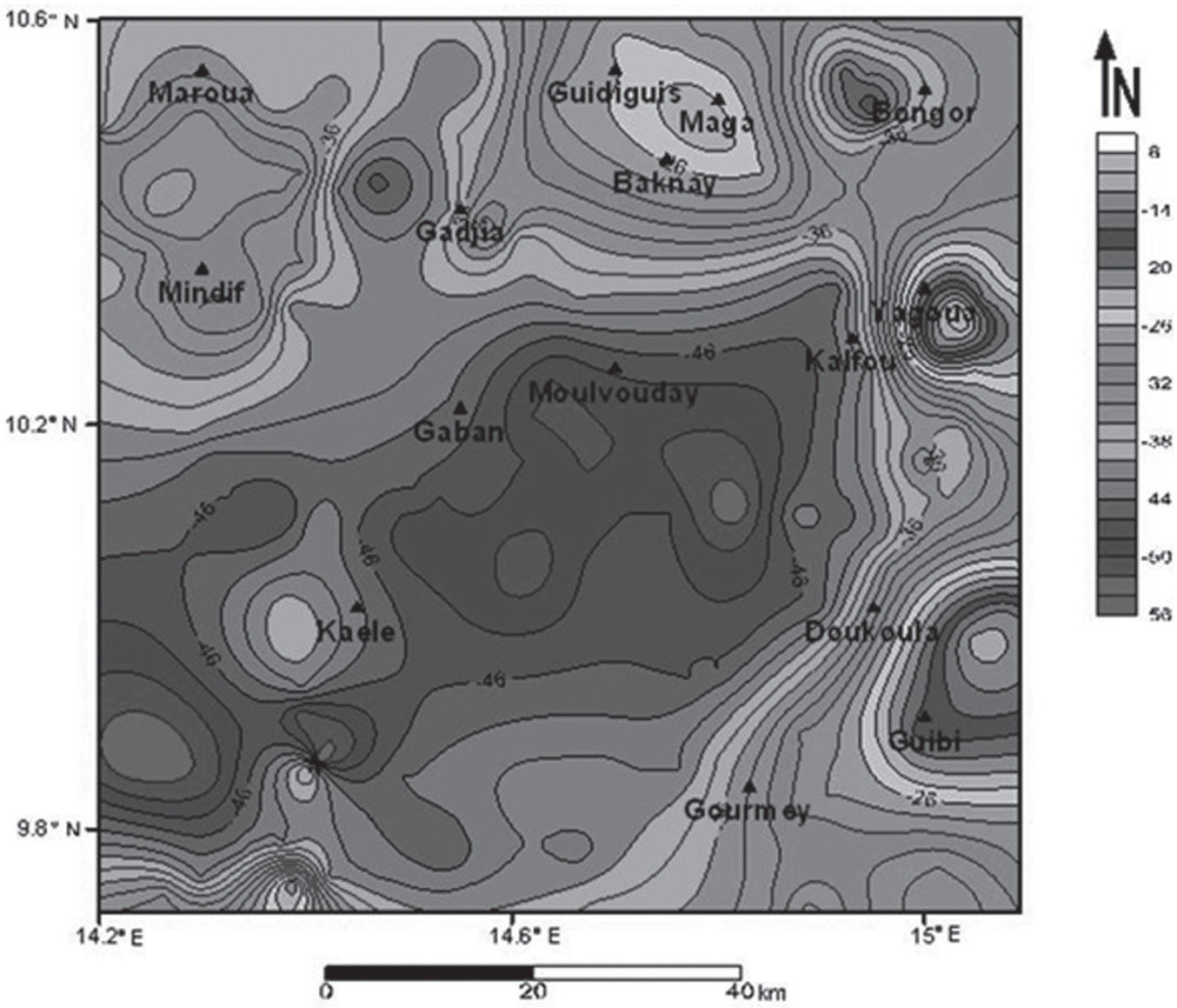
A new Bouguer map of Yagoua region

The new Bouguer anomaly map (Figure 8) obtained by the kriging method reveals several anomalies which can be grouped into two major families: a family of negative anomalies and a family of positive anomalies. The positive anomalies are located south of Kaele, at GuibiDoukoula, Yagoua, Guidiguis and at Maroua-Mindif. The positive anomalies of Guibi-Doukoula and Yagoua, observed on the new map, also appear in other documents. They appeared separated on Collignon (1968) but are absent on Louis (1970) and Poudjom et al. (1996) maps. The reappear clearly separated on the new map proposed by the current study. In addition, this map brings out the positive anomalies of Maga and MarouaMindif formerly reported by Collignon (1968) and absent on Louis (1970) and Poudjom et al. (1996) maps. By comparing these results (Figure 9) with the geological map (Figure 1) and, according to Manga et al. (2001), Njandjock (2004) and Njandjock et al. (2006), the positive anomalies of Guibi-Doukoula, Yagoua and Guididuis correlate with an uplift of gneissic-granite type dense materials. The positive anomaly of Maroua-Mindif correlates with Mindif’s “tooth” syenite block. The negative anomaly directed NE-SW extends from west Kaele to north Moulvouday and occupies the center of the study area. This negative anomaly is surrounded by positive anomalies and may coincide with a Quaternary sedimentary cover at Moulvouday. Compared to Manga et al. (2001) and Njandjock et al. (2006), this large anomaly may be the gravity signature of the MoulvoudayYagoua sedimentary basin.

Figure 8.

New anomaly Bouguer map of Yagoua region, 2012.

Conclusion

In this study, the experimental variogram was calculated from the existing gravity data. The RMS and the hindered points technique showed that the best theoretical variogram for these data were spherical. This variogram was therefore used to produce a new regular gravity data base and a new gravity map of the Yagoua region which can be used in further researches. This study includes mapping of the Moulvouday negative anomaly which may correlate with sedimentary thickening, while positive anomalies of Guibi-Doukoula and Yagoua may correspond to granite-gneiss dense basement material uplift. In addition, we confirm the positive anomalies of Maga and MarouaMindif which no longer appeared on Louis (1970) and Poudjom et al. (1996) but were reported by Collignon (1968). In addition, positive anomalies of Guibi-Doukoula and Yagoua that appeared separated on the Collignon map (1968), and which were present on the Louis (1970) and Poudjom et al. (1996) maps, reappear clearly separated.

Acknowledgements

We would like to thank Dr. Cinna Lomnitz and Mister ACHAKENG NKEMKA John of Ministry of Scientific Research and Innovation-Cameroon, for corrections and suggestions on the manuscript.