La solución analítica de las componentes del tensor gravimétrico, utilizando la ecuación del potencial gravitacional para un ensamble volumétrico compuesto de prismas de densidad constante, requiere un alto costo computacional. Esto se debe a que el potencial gravitacional de cada uno de estos prismas tiene que ser calculado para todos los puntos de una malla de observación previamente definida, lo cual resulta en una carga computacional de gran escala. En este trabajo introducimos un diseño híbrido y su implementación paralela basada en OpenMP y MPI, para el cálculo de las componentes vectoriales del campo gravimétrico (Gx, Gy, Gz) y las componentes del tensor gravimétrico (Gxx, Gxy, Gzz, Gyy, Gyz, Gzz).El rendimiento obtenido conlleva a óptimas relaciones del speed-up, ya que el tiempo de cómputo es drásticamente reducido. La técnica de paralelización aplicada consiste en descomponer el problema en grupos de prismas y utilizar diferentes espacios de memoria por núcleo de procesamiento, con el fin de evitar los problemas de cuello de botella cuando se accesa a la memoria compartida de un nodo del cluster, que se producen generalmente cuando varios hilos de ejecución acceden a la misma región en OpenMP. Debido a que OpenMP solo puede utilizarse en sistemas de memoria compartida es necesario utilizar MPI para la distribución del cálculo entre los nodos del cluster, dando como resultado un código híbrido OpenMP+MPI altamente eficiente con un speed-up prácticamente perfecto. Adicionalmente los resultados numéricos fueron validados con respecto a su contraparte secuencial.
The analytic solution of the gravimetric tensor components, making use of the gravitational potential equation for a three-dimensional volumetric assembly composed of unit prisms of constant density, demands a high computational cost. This is due to the gravitational potential of each one of these prisms must be calculated for all of the points of a previously defined observation grid, which turns out in a large scale computational cost. In this work we introduce a hybrid design and its parallel implementation, based on OpenMP and MPI, for the calculation of the vectorial components of the gravimetric field and the components of the gravimetric tensor. Since the computing time is drastically reduced, the obtained performance leads close to optimal speed-up ratios. The applied parallelization technique consists of decomposing the problem into groups of prisms and using different memory allocations per processing core to avoid bottleneck issues when accessing the main memory in one cluster node, which are generally produced when using too many execution threads over the same region in OpenMP. Due OpenMP can be only used on shared memory systems is necessary to use MPI for the calculation distribution among cluster nodes, giving as a result a hybrid code (OpenMP+MPI) highly efficient and with a nearly perfect speed-up. Additionally the numerical results were validated with respect to its sequential counterpart.
The shared memory architecture is becoming more common every day in the highperformance computing market. With the hardware technology advances allowing us to have a great number of cores with access to the same memory locations, nowadays it is not that expensive to have systems with forty or sixty cores using shared memory. OpenMP is now a standard for symmetric multiprocessing systems (SMP) (even can be used transparently in the Xeon Phi architecture (Calvin et al., 2013)) sustained by a combination of function and compiler directives, a standard for the symmetric multiprocessing (SMP) systems (Dagum and Menon, 1998; Curtis-Maury et al., 2008). OpenMP has proven to be a powerful tool for SMP due to several reasons: it is highly portable; it allows fine and medium granularity, each thread can access to the same global memory; and has their own private memory, and it also has a greater level of abstraction than MPI model (Brunst and Mohr, 2008).
MPI is a library supported on the Same Program Multiple Data (SPMD) model and on the message passing model, with an explicit control of the parallelism. The processes can only read and write in their respective local memories and the data in these memories is transferred through calls to functions or procedures which implement the message passing model. Among the principal characteristics of MPI are that it can run in architectures of shared and distributed memory, is convenient for medium to coarse granularity and that employment is widely extended, making it extremely portable among platforms (Krpic et al., 2012).
Using a hybrid programming model we can take advantage of the benefits of two programming models OpenMP and MPI. MPI is normally used to control the parallelism among cluster nodes, while OpenMP is applied in the creation of threads of fine granularity tasks within each node. Most applications developed in hybrid model involves a hierarchical model: MPI is for the higher level and OpenMP for the lower one (Smith, 2000).
One of the potential benefits of using hybrid model programming consists of getting rid of the barrier of scaling that each model has. Generally, in MPI the scaling is limited by the communications cost, because an application is affected by the overload of communication when the number of processes is increased. In OpenMP the performance of an application is affected by cache coherence problems and access to shared memory which may lead to bottleneck issues between the execution threads when trying to access memory. By mixing these methodologies of parallel programming (OpenMP and MPI), we can obtain a more diverse granularity of the application and therefore a better performance than by using each one on its own.
There are different applications which use this programming paradigm: OpenMP with MPI. For example, in the solution of sparse linear systems (Mitin et al., 2012), in graphcoloring algorithms (Sariyuce et al., 2012), in some models of fluid dynamics (Amritkar et al., 2012; Couder-Castañeda, 2009) and finite element methods (Boehmer et al., 2012), in the simulation of turbulent fluids (Jagannathan and Donzis, 2012), even in the simulation of combustion chambers (Környei, 2012) and the implementation of neural networks (Gonzalez et al., 2012). As can be observed, there are numerous computational implementations using OpenMP with MPI, nevertheless, this type of design is supported on a natural decomposition of the domain (CarrilloLedesma et al., 2013), based on data. For our particular problem, each one of the processing units accesses all of the computational domain points.
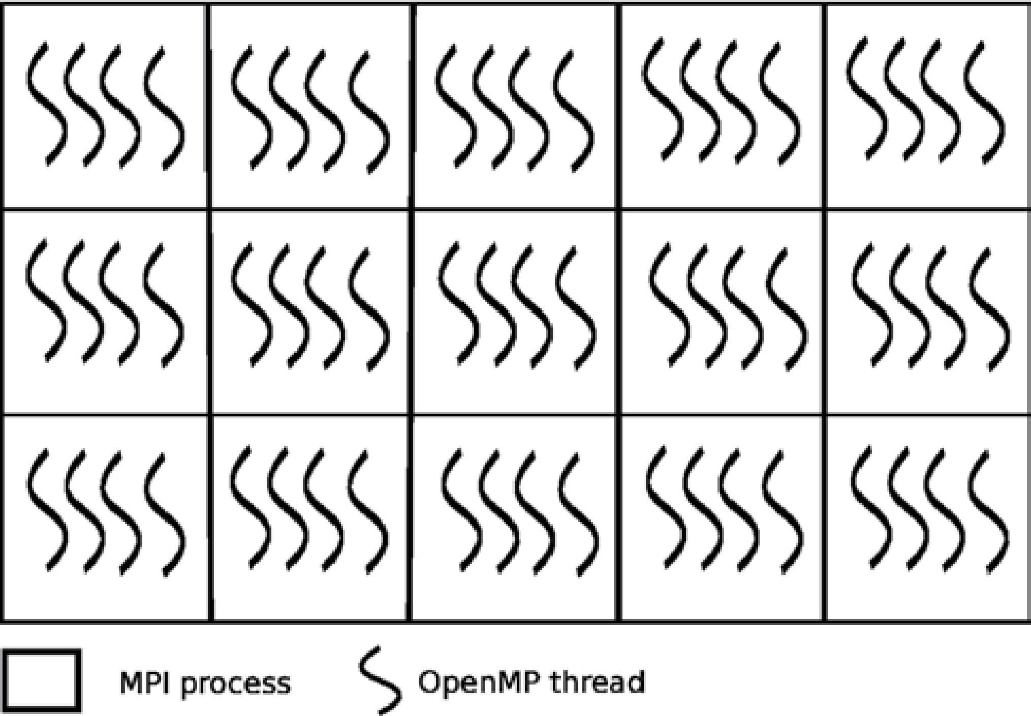
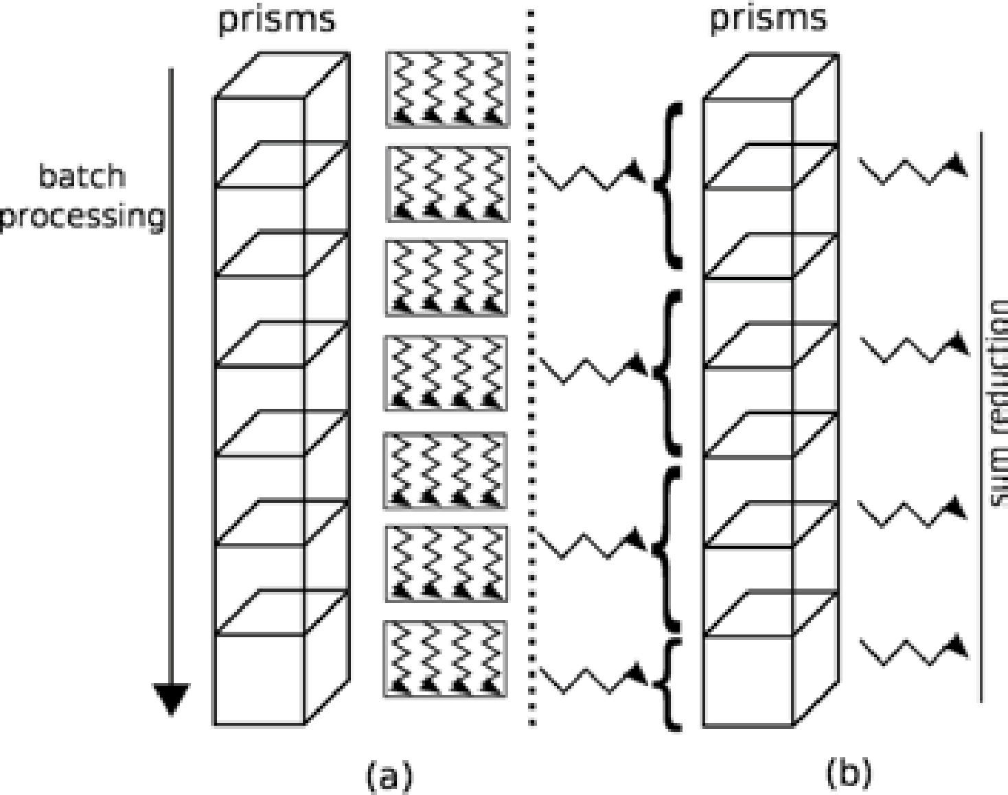
In Figure 1 is depicted a domain decomposition, where each task (process or thread) is given some data subset on which to work. This domain decomposition is commonly used for example in finite differences problems where computational domains divided disjointly among the different tasks.
On the other hand, in the direct conformation of gravimetric data, an initial model for the source body is constructed from geologicalgeophysical information. The anomaly of such model is calculated and compared to the observed anomaly, after which the parameters are adapted to improve the adjustment between them. These three steps that arrange the model properties — anomalies calculation, comparison and adjustment — are repeated up to the observed and calculated anomalies are similar enough.
A mass volume can be approximated by a set of rectangular prisms; if chosen sufficiently small, each prism can be considered to have a constant density. Because of the superposition principle, the gravitational anomaly of a body can be approximated at anypoint by summing the effects of all the prisms over that point. Even though this methodology appears simple (by reducing the size of the prisms to better adjust the source body), computing time is considerably increased. There are other approaching methods of the gravitational anomaly that can simplify the required computation (mass points or tesseroids approximations), however, they may complicate the construction of the geological model (Heck and Seitz, 2007).
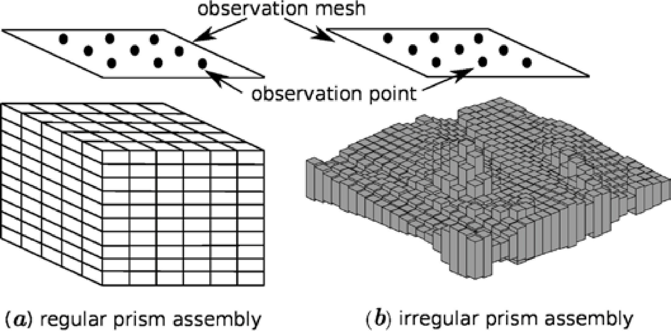
Application designThe application consists of calculating the gravimetric anomaly produced by a rectangular prismatic body with constant density with respect to a group of observation points (see Figure 2). The set of prisms is known as an ensemble of prisms, which is not necessarily regular. A set of irregular prisms can be configured as long as the prisms are not superimposed. Because the gravitational field complies with the superposition principle with respect to the observation points, if f is the calculated response at a point (x, y), then the observed response at the point f (x, y) is given by:
where M is the number of total prisms and ρ is the density of the prism.
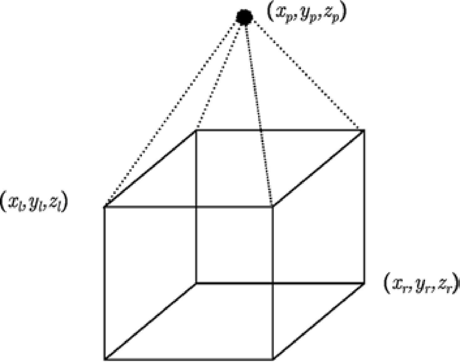
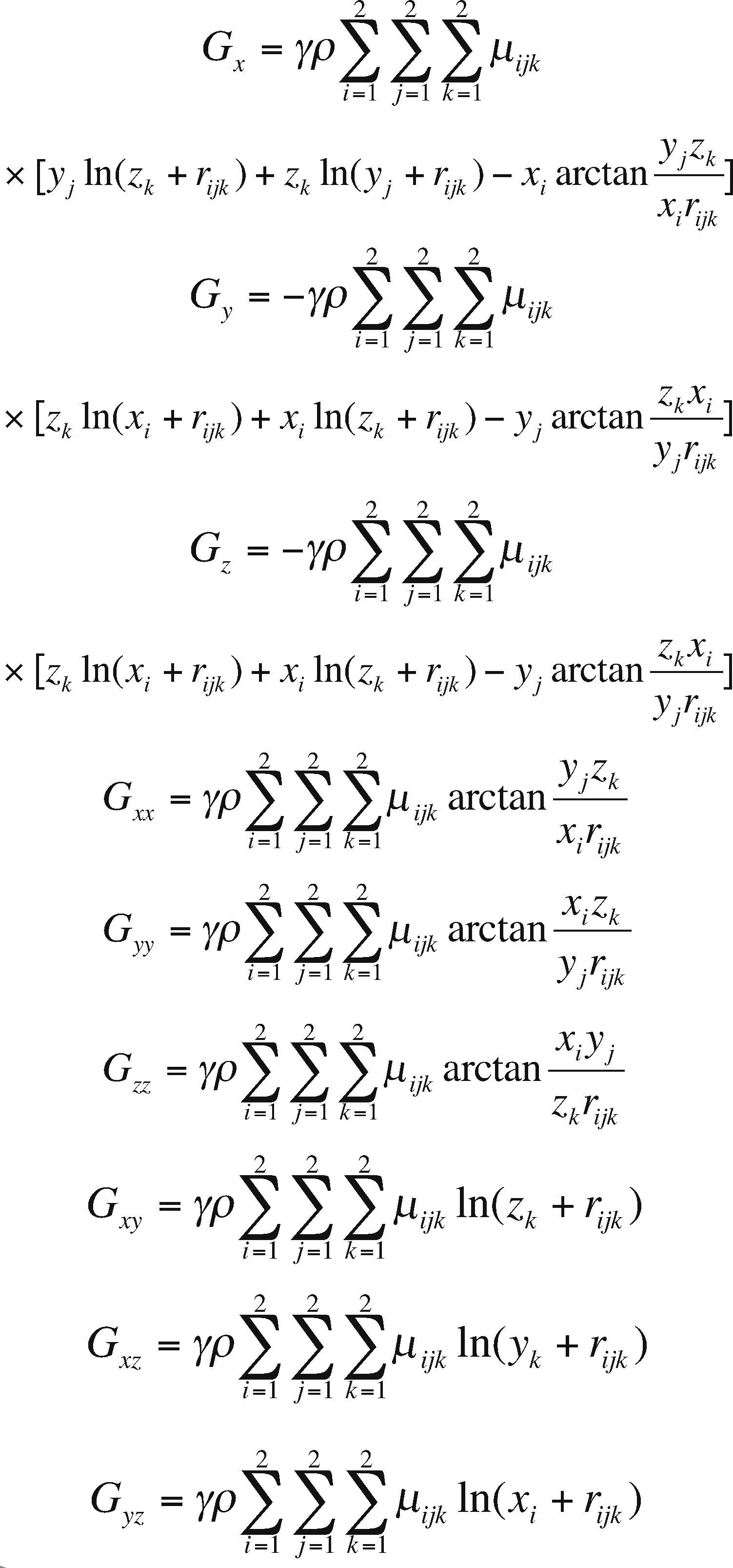
It is well known that the function that calculates the anomaly for a given prism from an observation point is written as follows (Nagy et al., 2000):
where (xl, yl, zl) is the top left vertex of the prism, (xr, yr, zr) is the bottom right prism and (xp, yp, zp) is the observation point and ρ the density, as shown in Figure 3.
The aforementioned is a large scale problem since, for example, a synthetic problem conformed by a set of prisms of 300 × 300 × 150 = 13,500,000 elements, against an observation grid of 100 × 100 = 10,000 points, results in the calculation of 135,000,000,000 integrals or differentials to solve the entire problem. The formulations we used are included in appendix A.
Computing time reduction in a numerical simulation is of great importance to diminish research costs. A simulation which lasts a week is likely to be costly, not only because the machine time is expensive, but also because it prohibits the quick acquisition of results to make modifications and predictions.
In many projects to be parallelized, several times the serial algorithm does not show a natural decomposition which allows easily porting it to a parallel environment, or the trivial decomposition does not yield good performance results. For such reasons it is convenient to use a hybrid programming methodology, as the one developed and presented in this paper. This methodology provides an adequate programming design to obtain a superior performance.
To develop a parallel program it is fundamental to search for the finest granularity, as in the methodology proposed by Foster (Foster, 1995). In this case it is possible to parallelize by prisms or by observation points. One of the requirements of the design is that it must be scalable, therefore the use of hybrid systems is quite appropriate; these systems are the most commonly used nowadays. Following Foster's methodology, it is necessary to begin with the finest granularity, in this case corresponds to OpenMP because it is in the lowest level. Subsequently the implementation follows with MPI, due to its coarse granularity.
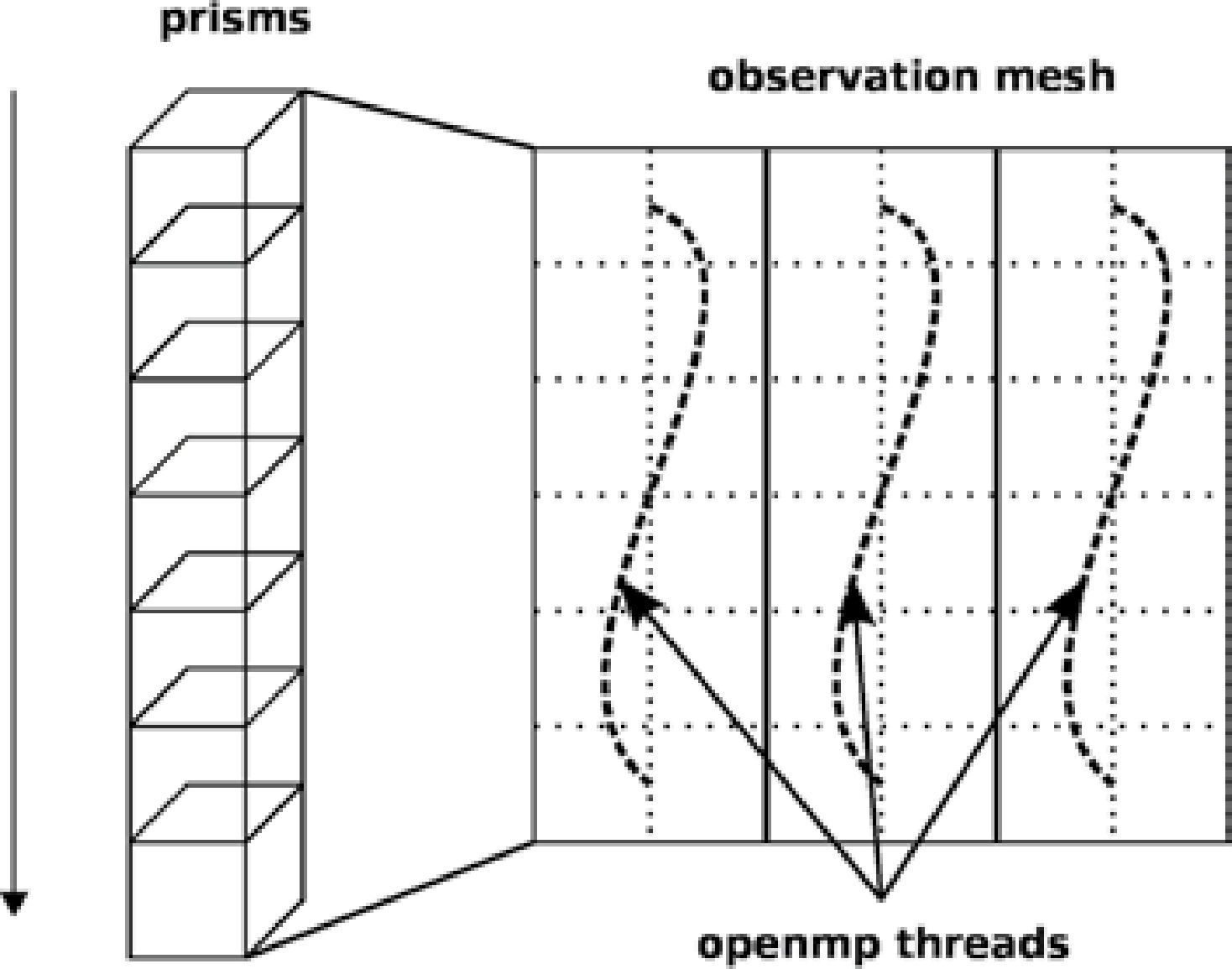
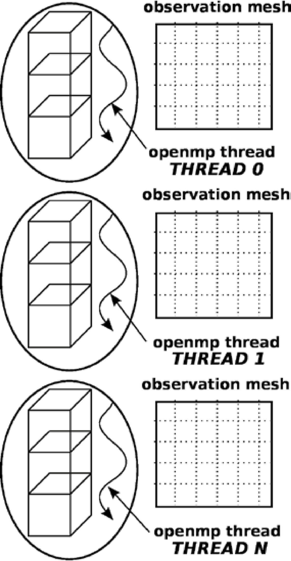
Implementation in OpenMPWe started our design with OpenMP because it handles shared memory and it is also the finest granularity. First we partitioned the domain into prisms, and for each prism we parallelized the calculation by observation points, as shown in Figure 4.
This parallelization by observation points is trivial and does not offer a great design challenge, since we simply partition the calculation with respect to the observation grid for each prism (see the pseudo-code 1). However, this scheme has several drawbacks. One of them is that the performance is not optimal since the number of prisms is much greater than the number of observation points. In other words, this partitioning is efficient as long as there are not too many threads working upon the observation grid, thus avoiding a bottleneck issue as a consequence of the threads works in the same memory allocation. Maybe the worst drawback lies in the fact that the parallel environment is created and closed, i.e. for each prism, a function which parallely calculates the anomalies is executed, but such environment is closed once the execution is over, and reopened for the following prism, which results in an unnecessary overload and therefore decreases the performance. Figure 5
Listing 1. Parallelization by observation points
For each prism from 1 to M
!$OMP PARRALLEL DO COLLAPSE(2)
For each j from 1 to Ny
For each i from 1 to Nx
G(i,j)=Gz(parameters)+G(i,j)
End For
End For
!$OMP END PARALLEL DO
End For
Listing 2. Parallelization by observation points
!$OMP PARRALLEL DO
For each prism from 1 to M
For each j from 1 to Ny
For each i from 1 to Nx
G(i,j)=Gz(parameters)+G(Thread, i,j)
End For
End For
End For
!$OMP END PARALLEL DO
The other parallelization option is to use prisms i.e., making the threads divide the work per number of prisms (see pseudo-code 2). To avoid the coherence problems of the cache it is necessary to create a different memory space for each execution thread, because it is not feasible to create a single memory space for an unique observation grid, shared by all the threads.
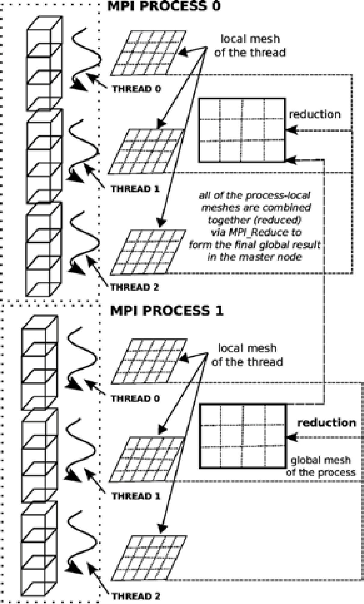
As observed in Figure 6, it is required to create an observation grid for each execution thread to avoid memory consistency problems. Bottleneck memory access issues are avoided since every thread writes in a different direction of the memory space. If only one grid were to be used, there would be access problems to the shared grid, which would create numerical inconsistencies.
One of the characteristics of OpenMP is that the computing is distributed in an implicit manner, therefore the partitioning of the M prisms, which composes the problem, is done automatically using a balancing algorithm included in OpenMP. In this case the decision is left to the compiler, which is optimum 99% of the cases (Zhang et al., 2004).
OpenMP+MPI ImplementationOne of the advantages of the prism parallelization is that it is easier to implement in MPI, producing tasks of coarse granularity using the same design previously applied in OpenMP. Having the observation grid partitioned would result in a more complicated and less efficient design using MPI. Since the parallelization in MPI is explicit, we need to manually distribute the number of prisms through a modular expression. If M is the number of prisms to calculate and p is the MPI process number (numbered from 0 to p−1), then for each process p we define the beginning and end of the prisms to be processed by p as pstart and pend, respectively. We define theinteger s as the quotient of the number of prisms M between the total number of processes pn and r as the remainder, the procedure to determine pstart and pend proceed as follows:
Therefore
and
If r ≠ 0 and p < r, then we adjust as:
and
If r ≠ 0 and p ≥ r, then:
and
This way we can distribute the number of prisms M over pn processes in a balanced manner; once this distribution is made, we can use the OpenMP implementation in each node. In other words, we occupy MPI to distribute the number of prisms in each node, and at the same time in each node we employ OpenMP to reduce the number of MPI processes, reducing communication time.
In consequence, the application is partitioned by the number of prisms M, both in OpenMP as in MPI. Another option is to parallelize by prisms in MPI and by observation points in OpenMP. Even though this is a viable option, it is not very scalable due the drawback discussed in the previous subsection.
Basically the design consists of allocating an observation grid per execution thread and a global observation grid in the master thread per computing node, subsequently the reduction of the sum of the grids per thread is done and stored in the global grid contained in the master thread, and finally at the end of the parallel calculation, every master thread will add their grid values to update the master thread of the master node using a MPI reduction method (see Figure 7).
It is necessary to mention that the implementation of the code was made with the FORTRAN 2003 specification, using as development tool the Intel Cluster Toolkit version 2013 of Intel Corporation.
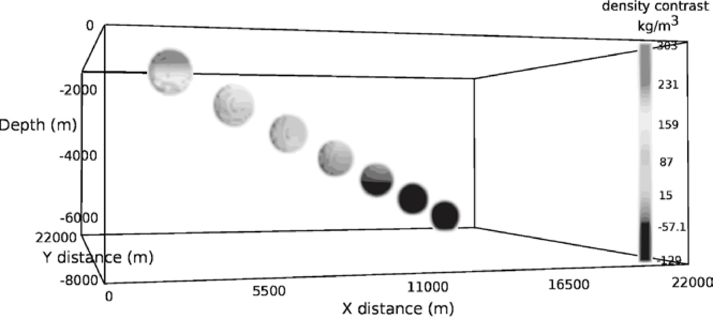
Performance experimentsFor the synthetic experiment we used a case composed by a cube of 700 × 700 × 50 prisms, with 7 contrasting spheres of variable density (see Figure 8). The spheres were conformed by 251,946 prisms and an observation grid of 150 × 100 = 15,000 points, to an elevation of 100 m. Therefore, the number of calls to a procedure required, to calculate the vector/tensor component of the gravity are 3,779,190,000; this classifies the experiment into a high-performance computing problem.
We tested the parallelized code by observation points versus the version by prisms using OpenMP. The first parallel scheme is technically easier to implement because for each one of the prisms the calculation of the cycles corresponding to the tracking of the observation grid is parallelized. The second scheme has a more complex implementation because it requires different space memory allocations. The performance experiments that calculate the components of the gravimetric tensor Gxx, Gzz, Gxy, Gyz using both versions were carried out in the server described below. We did not include the performance analysis for the vectorial components Gx, Gy and Gz, since its behavior is very similar.
The characteristics of the server where the tests took place with OpenMP are as follows:
- •
4 Xeon Intel (R) Xeon (R) E7-4850 Processors
- •
10 processing cores per processor
- •
Hyperthreading Technology deactivated
- •
512 GB of RAM memory
- •
Red Hat 6.3 as operating system
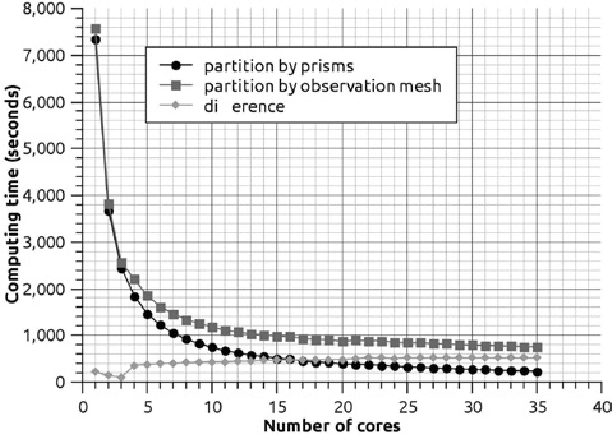
To interfere as least as possible with the processes of the operating system, we used 35 of the 40 cores available in the server. Initially we can say that the prisms implementation and with independent memory per core was 3.22X faster than its counterpart of observation points. Therefore, while the observation points version uses 757 s, the version partitioned by prisms only consumes 235 s.
The comparison of the computing times per thread in the partition by prisms against the partition by observation points is shown in Figure 9.
In Figure 9 it can be seen that the performance behavior is kept stable in both types of partitioning; however, by prisms the best reduction in time is obtained. To prove that the partitioning by prisms keeps reduction time practically linear, we graphed the speedup of the performance by prisms.
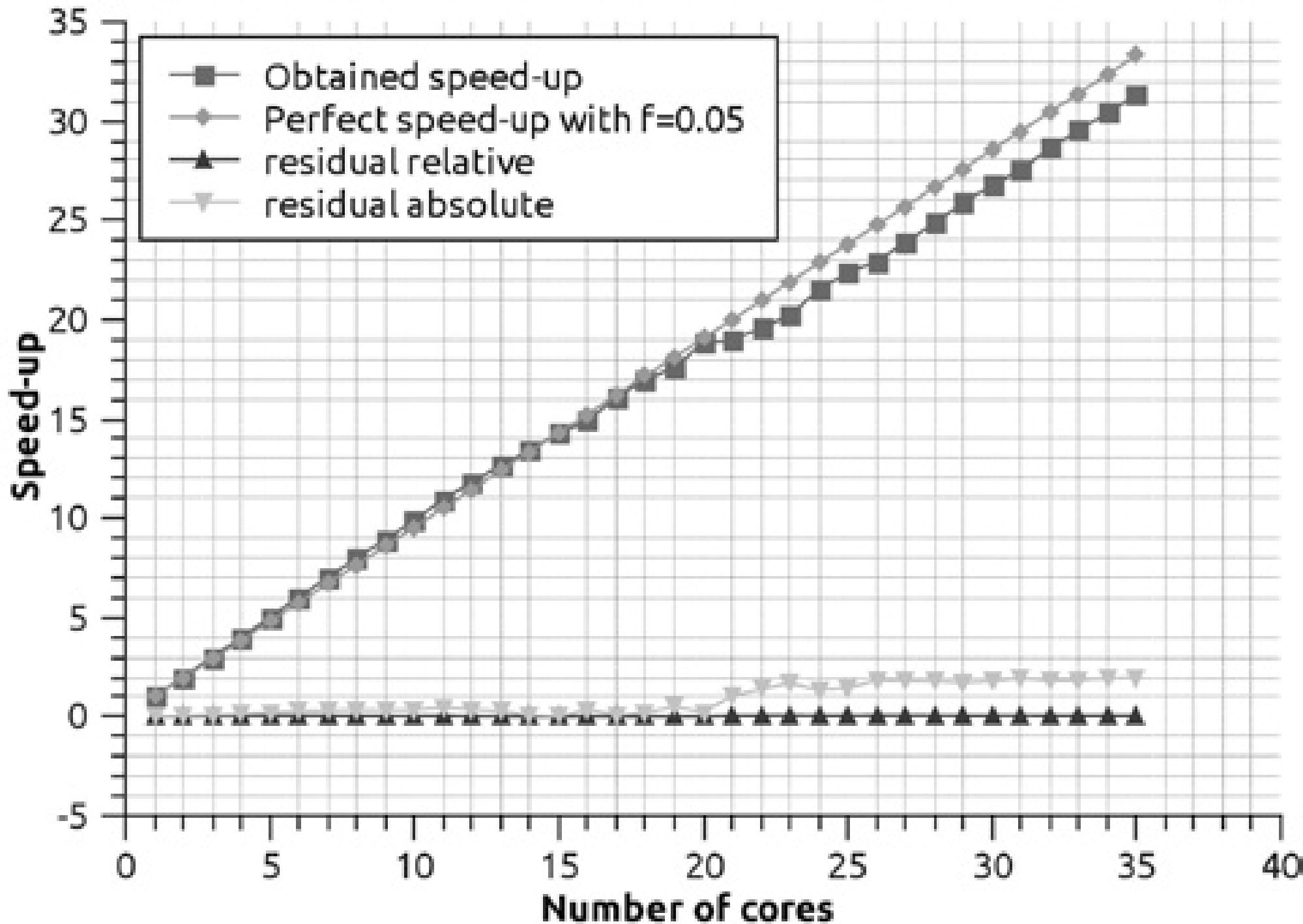
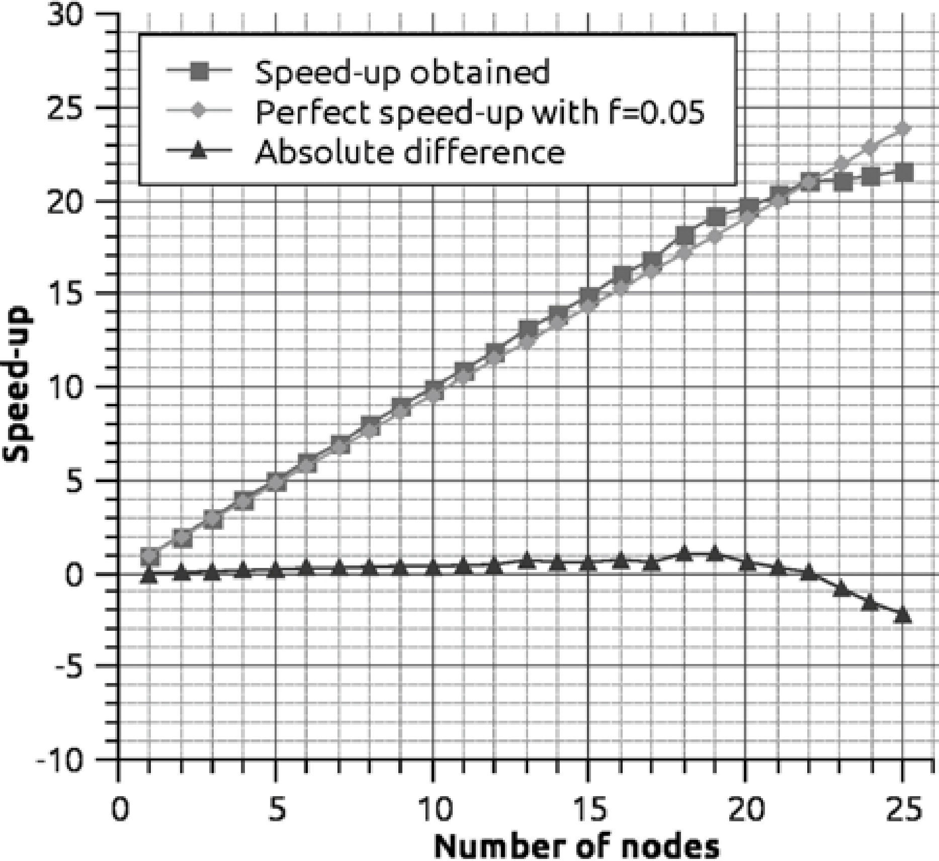
For the speed-up shown in Figure 10, we considered a serial fraction of 5% (f = 0.05). In this fraction the necessary reductions to sum the grid points for each core are contemplated, the total result of the anomaly is calculated as:
where, for each (i, j) Of is the final observation, Ot is the calculated grid by core t and Nt is the total number of cores. Therefore, we considered that 95% of the code is parallel, and according to Gustafson's law, the maximum textitspeedup that can be obtained with 35 processing units, in this case cores, is 35 + (1-35) × (0.05) = 33.30. The experimentally obtained speed-up result was 31.31, which represents an absolute difference of 1.99 and a relative difference of 0.06, which shows the efficiency of the implementation.
Another indicator which must be contemplated is the efficiency E, defined as:
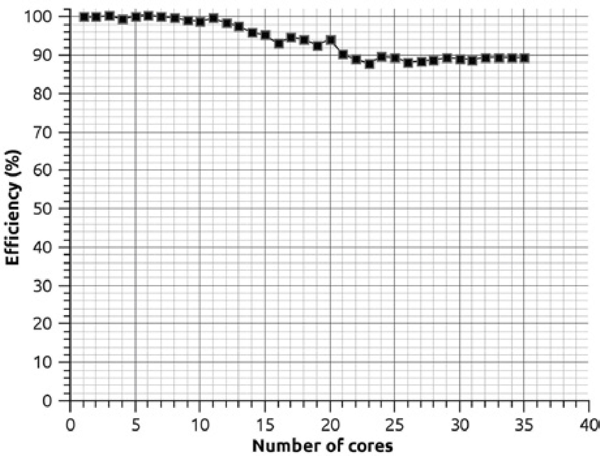
where S(n) is the obtained speed-up with n tasks, and indicates how busy the processors or cores are during execution. Figure 11 shows that the efficiency by prisms is high since on average every processing core is kept busy 94% of the time. The efficiency E also indicates that the partitioning by prisms is scalable, which means that we can increase the number of processors to improve time reduction while not losing efficiency in the use of many cores. The scalability must be contemplated as a good design of the parallel program since it allows scaling the algorithm, so we could expect when the number of processing units is increasing the performance is not affected.
The design using OpenMP is limited to architectures of machines of shared memory, therefore we are now making experiments using a hybrid machine commonly known as cluster, mixing OpenMP+MPI with the methodology described in subsection 2.2.
The characteristics of the cluster where the numerical experiments were carried out are as follows:
- •
Node: Intel(R) Xeon(R) model X5550 processors with four physical cores processor.
- •
44 processing nodes
- •
Hyperthreading Technology enabled
- •
40 GB of RAM memory per node
- •
Red Hat 6.3 as operating system
- •
InfiniBand 300Gbps
We started by evaluating the performance of each cluster node, as opposed to the experiments done with the 40 cores server, where hyperthreading technology (HT) was disabled. In this case HT is enabled, so each node reports the handling of 8 execution threads instead of 4, but we only have 4 physical floating point units (FPUs). Since our program is computationally intensive, we have to find out if we benefit from the use of HT; some studies have reported the use of HT in numerical applications can modify the performance by 30% (Curtis-Maury et al., 2008).
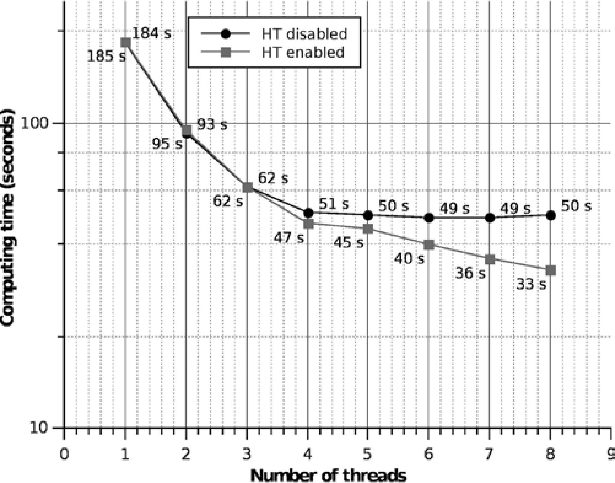
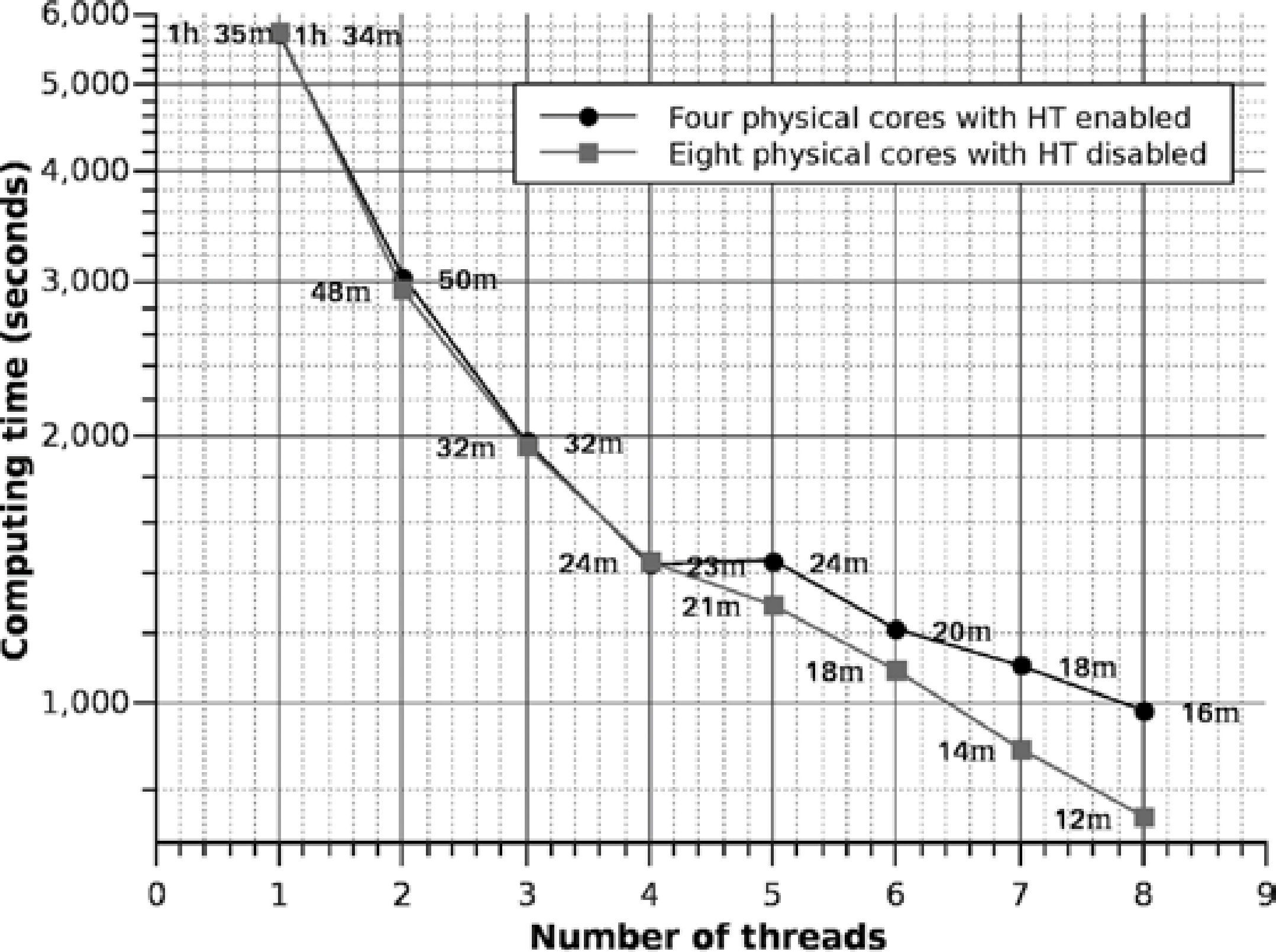
The behavior obtained using one node containing 1 processor with four real cores with HT enabled/disabled can be exposed by an analysis of the computing time graph, shown in Figure 12, the problems analyzed is setup with 13,997 prism conforming a sphere with a mesh of 150 × 100 observations points.
As can be observed, the best run-time performance that we can obtain from the processor in HT mode is not produced with 4 execution threads, the best performance is obtained with 8 threads, but the time is not doubly improved. This occurs since two threads share the same FPU and the HT technology is designed to quickly switch between threads, and therefore there is not a double improvement in time but the performance gain is approximately 30%, which means that the two threads make better use of the FPU,therefore is necessary to create two threads per core to obtain the maximum performance when the HT is enabled. When the HT is disabled we have an asymptotic behavior after 4 threads but did not reach the performance obtained using the HT mode.
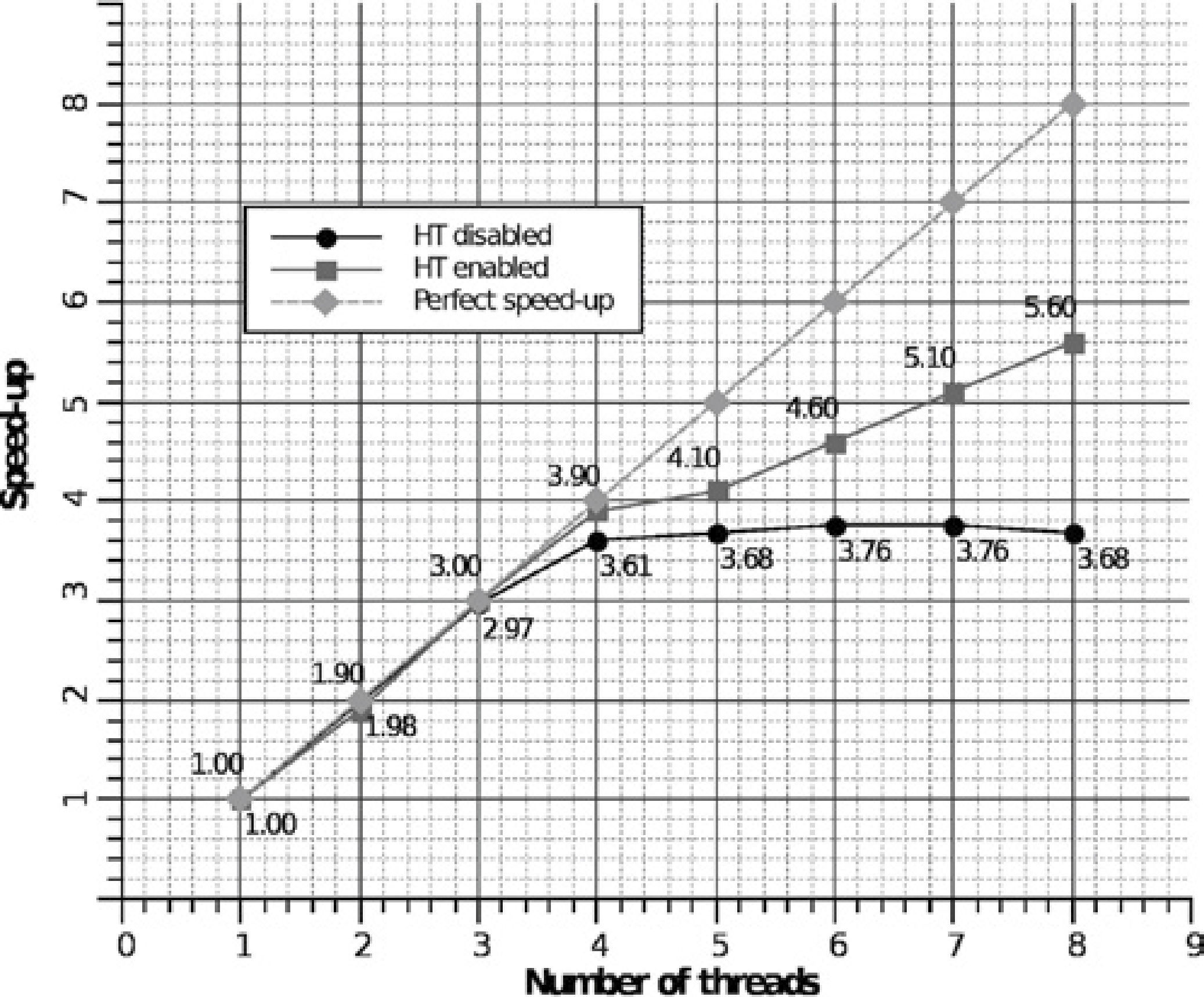
In Figure 13 it can be observed that when HT technology is enabled we obtain a linear speed-up up to 4 execution threads; this is obvious since there are only 4 physical FPUs. Nevertheless, with the HT we can have a better use of the FPUs improving the speed-up up to 5.60, this is, 1.6 more processing units. With the HT disabled, a similar performance is observed up to 4 threads, although this performance is below the one with the HT enabled. For more than 4 threads, the performance with the HT disabled begins to decrease.
Speed-up using only one node with HT enabled/disabled corresponding to the execution times shown in the Figure 11.
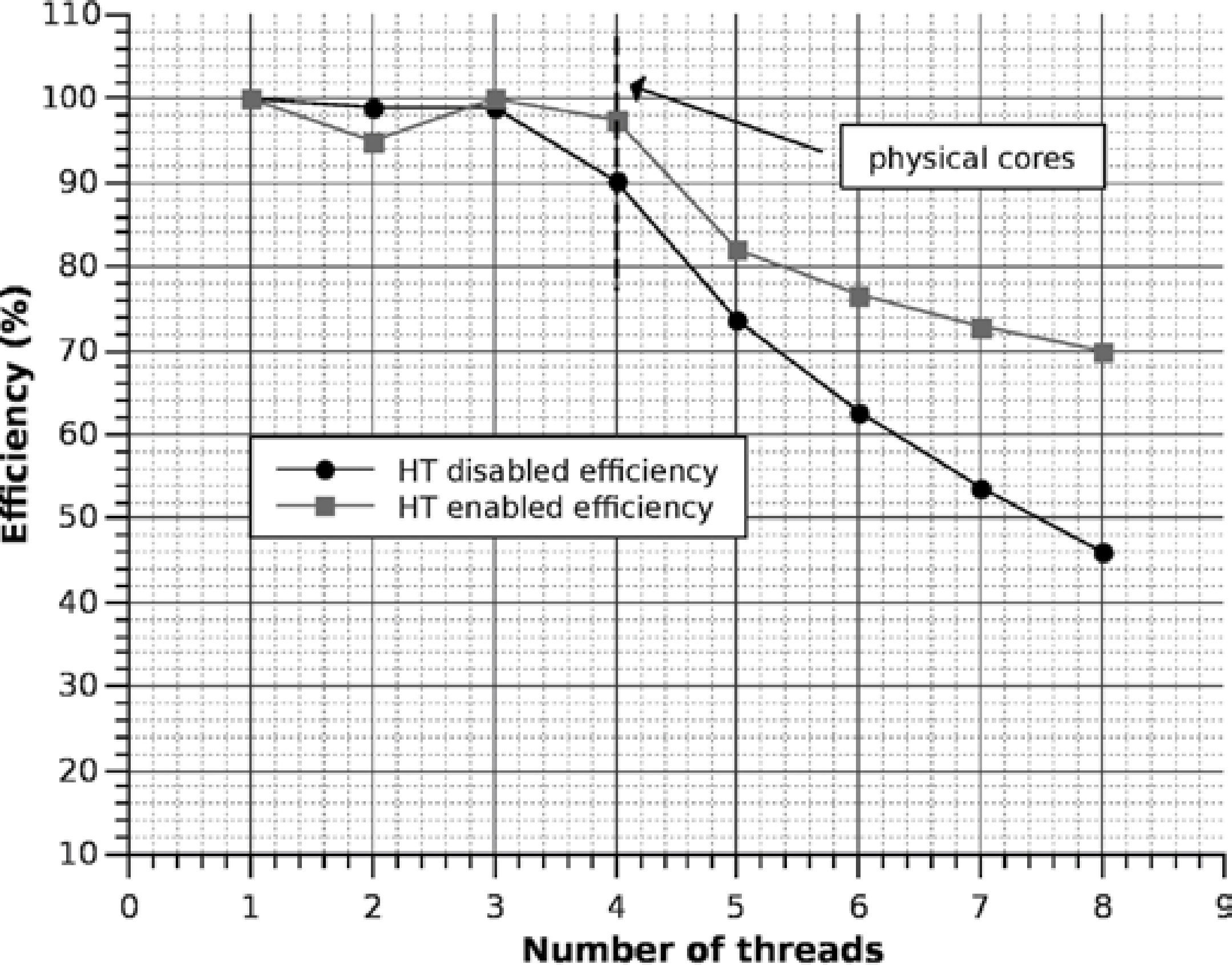
The efficiency corresponding to the speedup shown in Figure 13 is graphed in Figure 14; notice how HT is able to increase the efficiency of some intensive floating point applications up to 30% when the number of threads equals the number of physical cores. Of course, the best efficiency is obtained with 4 threads because we have 4 FPUs, nevertheless we can get a better performance creating 4 threads more using the additional virtual processors created by the HT.
To analyze the performance in a node with the original problem (shown in Figure 8), we added a processor in the second socket to one of the nodes. In other words, we created a node with eight real cores to compare it against a node with four real cores with HT enabled. The results of execution time are shown in Figure 15.
Eight real cores with HT disabled vs four real cores with HT enabled for the problem setup in the Figure 8.
It must be taken in consideration our cluster nodes are composed of a single processor with HT enabled, we only added another processor in the second socket to a node for experimental purposes. To have a better perspective of the performance, we determined the speed-up through both node configurations we showed in Figure 16. A nearly perfect speed-up can be observed for the node with 8 real cores, but a increase of 1.8 processing units for the node with 4 real cores with HT enabled. Evidently, if we enable HT in the machine with 8 real cores we would have 16 reported processors, and to get its maximum performance we would have to create 16 threads. However, the experimentation with 8 real cores was only for comparisonpurposes, since the cluster configuration is made of one node with 4 real cores with HT enabled. It can also be observed that each node of the cluster reduces the time by a factor of 5,8X against the serial version.
Eight real cores with the HT disabled vs four real cores with HT enabled for the problem setup in the Figure 8.
Once it is known that the best node performance is achieved with 8 execution threads for a node with 4 real cores with HT enabled and with the partition by prisms, we can consider each node as a processing unit and distribute the computing with MPI, obtaining a code with a hybrid programming model.
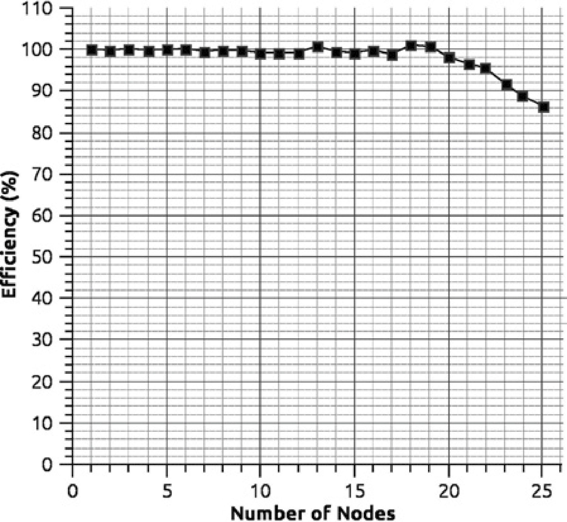
The speed-up results using 25 cluster nodes are displayed in Figure 17; a serial fraction of 5% (f = 0.05) is considered since in MPI there needs to be reductions in the sum for each node. The results show that a nearly perfect speed-up is obtained up to 22 nodes. From this point on, the speed-up starts declining because the application performance is affected by the communication time between nodes. In other words, the granularity of the tasks begins to decrease for this problem of 249,946 prisms for 30 nodes. This implies that by increasing the granularity of the problem (increasing the number of prisms), the speed-up is also increased until it becomes stable, to decrease again later on.
The efficiency graph related with the speedup of Figure 16 is shown in Figure 18. Notice how the efficiency is below 90% after node 23. If we consider that we have an increase in speed 5.8 times per node (from Figure 15) with respect to the serial version, then the optimum speed factor for this cluster (for a problem of 251,946 prisms) is approximately 5.8 × 22 = 127.6X, i.e. 127 times faster than the serial version. Obviously, as previously stated, if we increase the granularity (number of prisms), the efficiency increases as well. In fact, we reduce the computation time of the spheres problem from 1h 34 m 56 s to 34 s
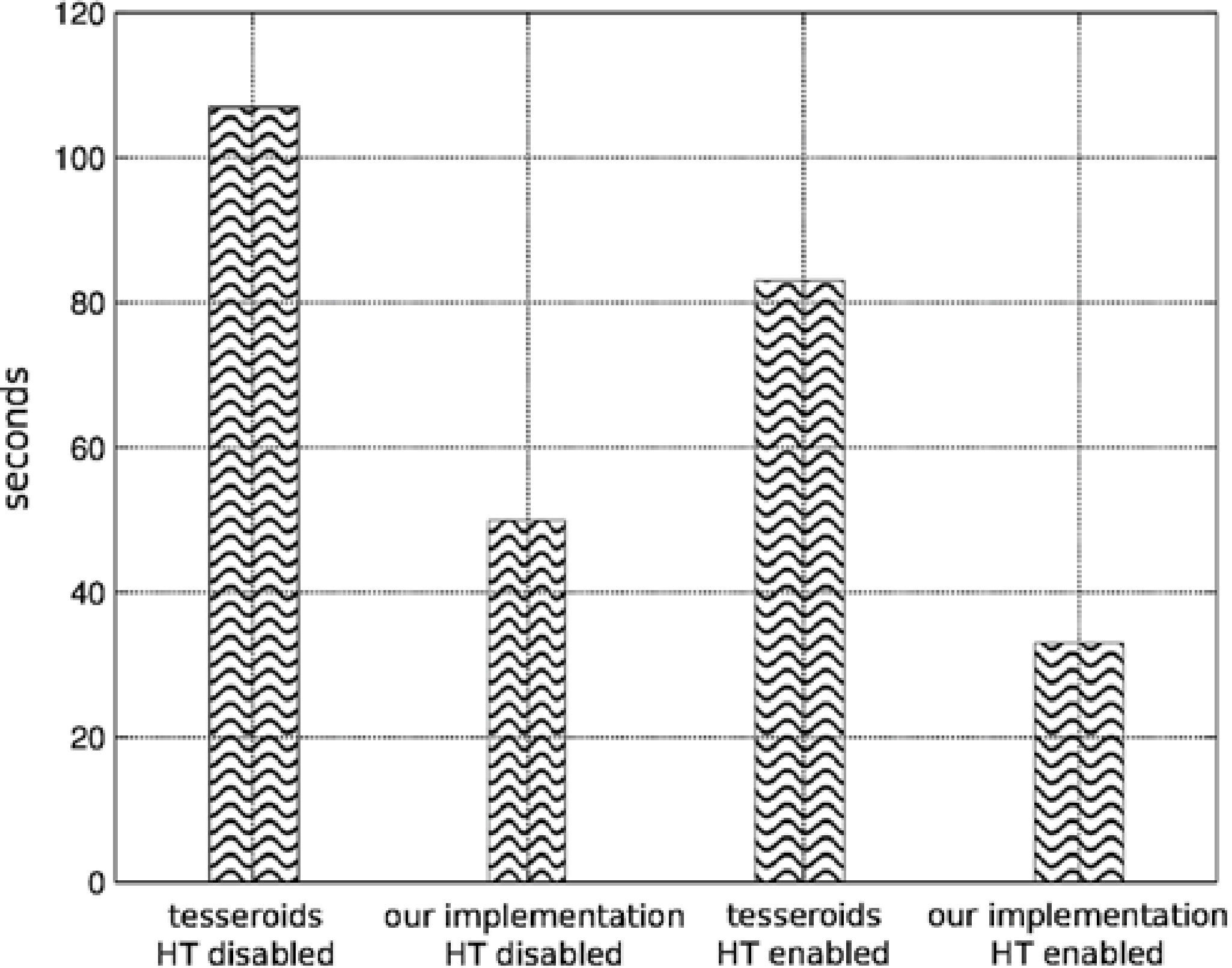
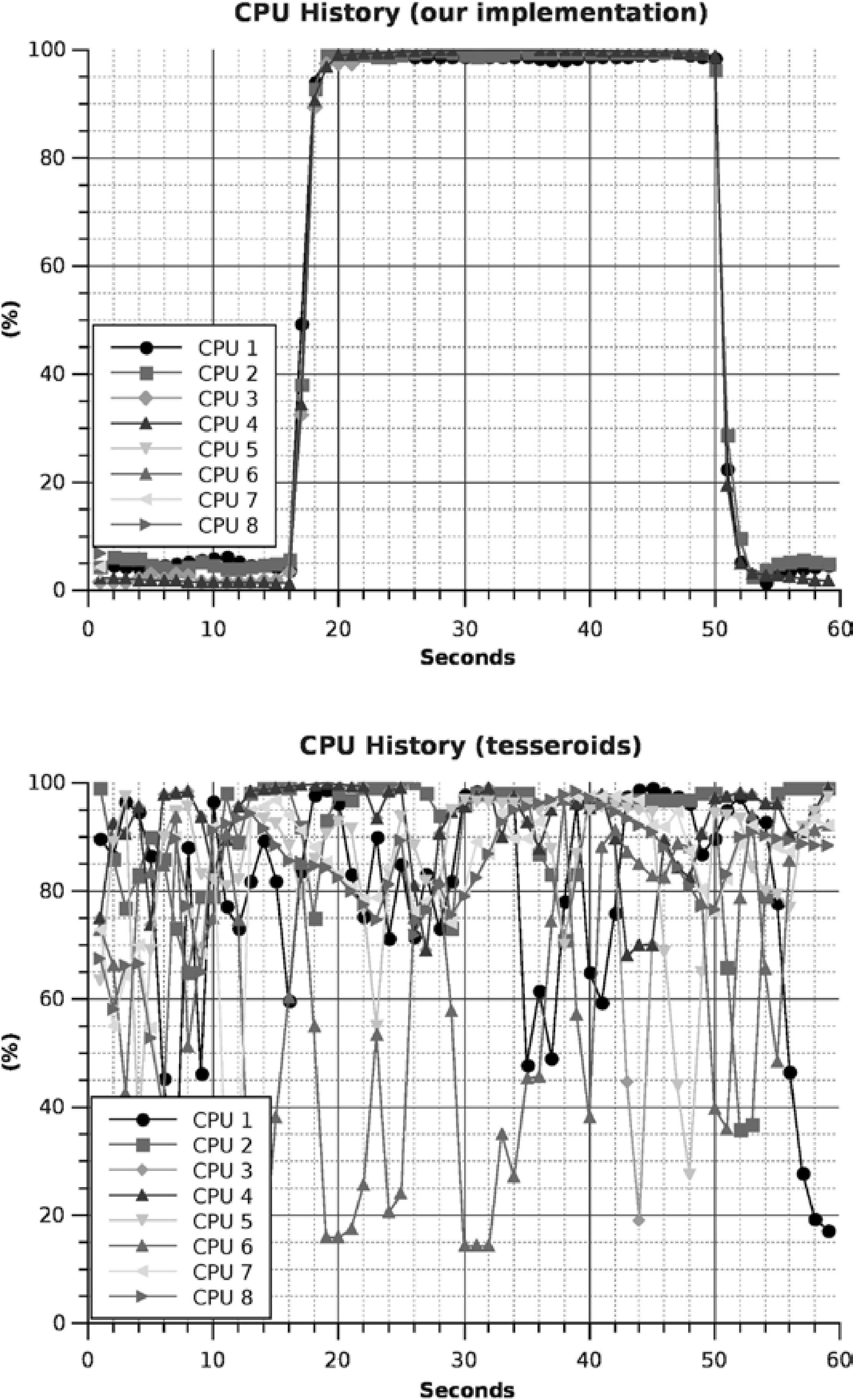
Comparison with similar programsTo provide a better perspective of the obtained performance with the parallel implementation of our code, we compared against an open source code called tesseroids (Uieda et al., 2011), which can be downloaded from/dx.doi.org/10.6084/m9.figshare.786514. We chose the problem of 13,997 prisms which form an sphere against 10,000 observation points, since tesseroids is not distributed (can not be executed on a cluster) and can only accelerate the computation in shared memory machines. The execution times are shown using the bar chart in Figure 19, where it can be observed that with HT disabled we have a speed improvement of 2.14X and with HT enabled of 2.51X with respect to tesseroids. This performance improvement is due to our program design takes a better advantage of the processor technology and keeps the cores occupied to the maximum by using a prisms parallelization scheme based on different memory allocations. This can be observed in the CPU history graph shown in the Figure 20.
Numerical code validationThe main challenge of the parallel programming is to decompose the program into components which can be simultaneously executed to reduce computing time. The decomposition level is highly influenced by the type of architecture of the parallel machine. In this case the design was made with a hybrid programming strategy to get the maximum out of the architecture. Although the reduction of the execution time is the main objective of the parallel programming, the validation of the code is a topic that should be covered since inherent parallelism programming errors can occur.
To measure the error, we compared the previously validated sequential counterpart in the synthetic experiment with the analytical solution. We used the L2 norm error or RMS (Mickus and Hinojosa, 2001; Menke, 1989), defined as:
where gi,jp is the tensor component, parallely computed, and gi,js is the serially calculated component.
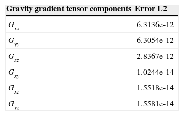
In Table 1 the errors of the gravimetric tensor components are shown, parallely calculated with respect to the serial form.
From the errors obtained it can be noticed that there is no numerical difference, therefore the parallel version is correctly implemented.
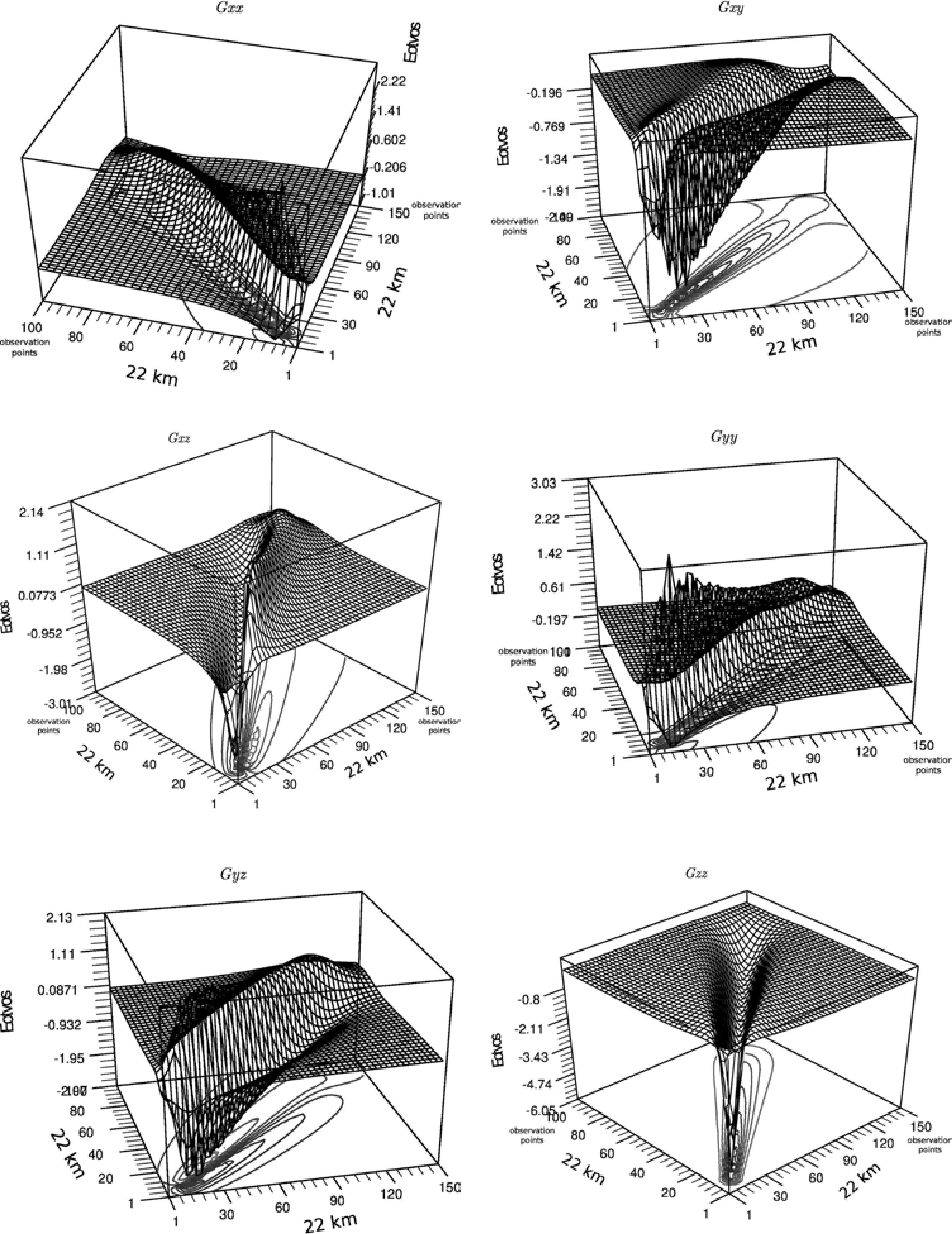
The surface graphs of the gravitational fields are shown in Figure 21. These graphs correspond to the components of the gravimetric tensor, calculated for the synthetic case studied in Figure 8.
ConclusionsA parallel design for the calculation of the vectorial and tensorial components of the gravity anomaly was implemented and validated using a hybrid methodology with OpenMP and MPI. The numerical experiments and the obtained indicators validate that the implementation is very efficient and that it also yields good results with respect to the numerical solution.
We show that using the simplest or most trivial parallelization form does not contribute to the attainment of the best performance or the greatest exploitation of the platform. For our case, even though the partitioning by prisms requires a greater investment in the design and implementation, it was the most advantageous with respect to performance.
The HT technology could improve some numerical intensive applications up to 30%, nevertheless, to get the best performance it is necessary to create two threads per core when the HT is enabled.
We also conclude that this design can serve as a benchmark for solving problems which require the parallelization of schemes where the decomposition of the domain is not trivial or is shared by the processing units, as is the case of the observation grid. Finally the correct exploitation of OpenMP and MPI, jointly, can become a fundamental tool for parallel programming in clusters.
Future workAs future work we pretend to implement the code in CUDA NVIDIA with TESLA technology and compare these results with the cluster performance results presented in this paper, as the measurement of the error introduced by CUDA in single and double precision. The implementation in CUDA is a work of interest since the reduction of the variable values in CUDA technology is very complicated when used in shared form, as is the case with the observation grid.
The authors thank the support provided by the Mexican Institute of Petroleum (IMP, www.imp.mx) in allowing access to its computing equipment, as well as the financial support through project Y.00107, jointly created by IMP-SENER-CONACYT number 128376. Also, we would like to express our gratitude to the two anonymous reviewers for their helpful comments.
The Earth's gravitational potential G is a scalar quantity, its shape can be constrained by its slope in the x, y and z directions, called the gravitational attraction Gx, Gy and Gz (gravity vector field). In this work, we have investigated how to parallelize the analytical calculation of the components of the gravity field vector and the gravity gradients represented by a nine component tensor, because of the symmetrical or irrotational attribute, the gravity gradient tensor is reduced to only six independent components: Gxx, (the vertical gravity gradient), and For the right rectangular prism model, the analytical formulae for the three components vectors and the six gravity gradient components, corresponding to the Eq. (2) are given by:


