QVOA techniques for fracture characterization

Resumen

Se desarrollan nuevas técnicas de cálculo en el análisis del factor de calidad frente a la distancia fuente receptor y el acimut (QVOA) para caracterización de fracturas. Estas técnicas se aplican a datos sintéticos superficiales de reflexión con ruido.

Abstract

New computational techniques of QVOA analysis (Quality factor Versus Offset and Azimuth) for fracture characterization are developed. The techniques are applied to synthetic surface data of reflection with noise.

Introduction

Quality factor Q is a seismic characteristic of attenuation property of a medium. By the value of Q-factor, one may estimate what kind of liquid fills pores of the medium (a reservoir characterization), because the attenuation of reservoir is due to presence of a liquid in the pores. For estimating factor Q, many different computational methods have been suggested (e.g., Tonn, 1991; Quan & Harris, 1997; Dasios et al., 2001; Zhang & Ulrych, 2002), as well as methodologies of its application to real data (Dasgupta & Clark, 1998).

QVOA analysis (Q-factor Versus Offset, and Azimuth) was first intended by Chichinina et al. (2004, 2005). Then it was further developed by Chichinina et al. (2006a, 2006b, 2006c), and Zhu and Tsvankin (2006). In fractured anisotropic media, anisotropy of Q is present (Clark et al., 2001; Chichinina et al., 2004, 2005). Namely, the value of quality factor Q depends on offset and azimuth. An approximate formula of this dependence was first suggested by Chichinina et al. (2006a, 2006b) for transversely isotropic media with a horizontal axis of symmetry (HTI), as well as an idea to apply it to estimation of principal fracture directions. Formulation of the QVOA analysis by Chichinina et al. (2006b) is similar to formulation of AVOA analysis (Amplitude Versus Offset, and Azimuth) by Rüger (1998) which gives good results in fracture characterization for media without attenuation (Sabinin & Chichinina, 2008).

Here computational techniques of QVOA analysis for estimation of fracture directions are suggested. Some of them are developed by analogy with known AVOA techniques (Mallik et al., 1998; Jenner, 2002). The others are original.

The QVOA techniques deal with estimating an attenuation factor (or quality factor Q) in surface data of reflection, what is not a trivial problem. Methodologies of such estimation of Q are proposed by Behura & Tsvankin (2009), Shekar & Tsvankin (2011), Reine et al. (2012), and Sabinin (2012).

Estimation of a symmetry axis angle by QVOA

Attenuation of wave amplitudes due to dispersion obeys a law (e.g., Tonn, 1991):

where r is a travel distance, and β is an absorption coefficient.

Quality factor Q is defined (e.g., Sheriff, 2002) as the ratio of 2π times the peak energy to the energy dissipated in a cycle:

It relates to β as follows (Futterman, 1962):

where d=βrτf, f is frequency, and τ is travel time. For large values of Q, the approximation Q=πd is valid.

Let us define the attenuation factor α as

Value α varies between 0 and 1.

For a model of viscoelastic media with complex stiffness tensor, Carcione (1995) defined the formula 2πQ=Im[V2]Re[V2] where V is the complex velocity, which was used by Chichinina et al. (2006a, 2006b). This definition is valid only for large Q values. In the general case, following the definition of Q (Equation 2), it must be

For anisotropic media with attenuation, from (5), by following Chichinina et al. (2006b), one can describe a dependence of the attenuation factor on a wave-ray travel (incidence) angle θ, and on a source-receiver azimuth ϕ by the approximate formula:

where (Chichinina et al., 2006c)

A, B₀, C₀, are constants, provided B_{0 >} 0 for HTI media (Chichinina et al., 2004, 2006c), and ϕ₀ is the symmetry axis angle, usually unknown, which has to be estimated.

The incidence angle θ has a sense of the angle between axis z and the wave ray in the anisotropic medium with attenuation. The approximation was made under the assumption of a small value of sin⁶θ, which practically means: sin²θ <0.36, or θ <37°.

Numerical methods for estimating the symmetry axis angle

One can compute the value α in the target anisotropic layer with attenuation from seismograms of P-waves reflected from the top and the bottom of this layer (see next section). Usually, the data used are 3D seismic data from spaced receivers and sources within nodes of a rectangle grid at the surface. The symmetry axis angle is usually obtained for a square surrounding a node of the grid (for a bin), by using seismic traces which Common Middle Point (CMP) is within this bin. If such traces are few, then neighbor bins are combined into a superbin, and calculations are made for it. Therefore, a preliminary stage of the estimation is a selection and an extraction of seismic traces of the superbin from the 3D data.

All methods described below are applied to the individual superbin. Let the superbin have n traces (i = l,..., n) with incidence angles θ_i in the target layer and azimuthal angles ϕ_i^.

The first two methods use also sectoring; i.e., the traces of the superbin are sorted into m azimuthally equal sectors (j = l,..., m), with k_j traces in each sector, with incidence angles θ_k (k = l,..., k_j) in the target layer. It is adopted that all traces in the individual sector j have the same value of azimuth ϕ_j, equal to the middle azimuth of the sector.

Approximate method of sectors (ASM)

It is the most computationally simple method based on the idea by Mallik et al. (1998) for the AVOA. From (6) one can write for the sector j:

where α_jk is the value of α calculated from the trace k in the sector j.

Having α_jk and θ_k for all k in the sector j (k_j≥3), one can calculate A_j, B_j, and C_j from (8) by the least-squares method (e.g., Sabinin & Chichinina, 2008). These calculations have to be made for all sectors.

The unknown value ϕ₀ may be obtained from the first of equations (7) written for each sector j:

As a rule, B_j is calculated with errors incorporated by the least-squares method from the data. Equation (9) is valid only for precise, theoretical values of B_j, and reasonably can be replaced by another. Let Bj=Bj(p)+δj, where Bj(p) is the precise value, and δ_j is an error. Then equation (9) can be replaced by the following approximate equation, which is proved to be more convenient for calculations:

If the error δ_j is not large, then a and b must be close to each other for an HTI medium (a ≈ b), although generally saying a ≠ b.

System (10) has three unknowns (a, b, and ϕ₀), therefore m should be at least 3 for obtaining a solution. It is the same system as in the AVOA technique by Sabinin & Chichinina (2008). System (10) is solved by the least-squares method, and has two solutions (two ϕ₀ differing by π/2 with the same b but of opposite sign). The condition b > 0 may be used to distinguish symmetry-axis and fracture-strike directions (see Equation 7).

Method of sectors (SM)

It differs from ASM by the method of solving the azimuthal problem (9). Instead of the approximate equation (10), equation (9) is written in its precise form:

where ξ_{j =} cos²(ϕ_j– ϕ₀)

This simplification leads to a more complicated solution. Let us consider the functional of error

Functional F must be minimized over parameters b and ϕ₀. For this, it is necessary to solve the system of two equations:

Transformation of (13) gives the following nonlinear equation for obtaining ϕ₀^:

whereA=1m∑j=1mξj2,B=1m∑j=1myjξj,C=1m∑j=1mξjBj,D=1m∑j=1myjBj,andyj=sin[2(φj-φ0)].

Additionally, b = C / A

Equation (14) is trigonometric non-linear and is solved by the method of half-dividing. It usually has more than one solution for ϕ₀. From these solutions, one chooses the one that gives the minimum for the functional (12). This choosing can be erroneous for highly noised data.

Approximate truncate method (ATM)

This method is similar to Jenner (2002) for the AVOA. The sectoring is not needed. Equation (6) is truncated for simplicity, and it is combined with (10), as in ASM. It gives after transformation:

where α_i is the value α calculated from the trace i of the superbin.

If we define s_i = sin²θ_i^,S = sin(2ϕ₀), C = cos(2ϕ₀), g_i = cos(2ϕ_i), and h_i = sin(2ϕ_i), then equation (15) can be rewritten into a more convenient form as:

The values s_i, g_i, and h_i are known because they can be calculated from the headers of the seismograms and the parameters of the medium.

Let us consider the functional of error

Functional F must be minimized over parameters a, b, d, and ϕ₀. For this, it is necessary to solve the system of four equations:

The solution of system (17) gives the equation for obtaining the parameter ϕ₀:

where A1=a1b1-a22,B1=a1c1-a32,

A₂ = a₁b_{2 −} a₂a₃, H₁ = F₂a₁ − F₁a₂,

H₂ = F₃a₁ − F₁a₃, a₁ = B − A², b₁ = I − D²,

c₁ = J − E², a₂ = G − AD, b₂ = K − ED,

a₃ = H − AE, F₁ = f₁ − Af₀, F₂ = f₂ − Df₀,

The other parameters are:

and a = f_{0 −} bA − dCD − dSE

From (18), one can see that the solution ϕ₀ has a period of π2. This value of the period means that we must use an additional condition for understanding which value of ϕ₀ is the symmetry-axis azimuth. Application of the method has shown that the condition b > 0, as by analogy with ASM, fails sometimes.

Truncate method (TM)

This method differs from ATM by using equation (11) instead of (10). It leads to the following equation for superbin instead of (15):

where ξ_{i =} cos² (ϕ_{i −} ϕ₀).

In order to solve (19) by the least-squares method, let us consider the functional of error

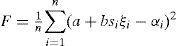
Functional F must be minimized over parameters a, b, and ϕ₀. For this purpose, it is necessary to solve the system of three equations:

Transformation of (21) gives the non-linear equation for obtaining ϕ₀:

where A₁= AF₁– BF_0’B_{1 =} AF₀– F_1’

Additionally, b = B₁ / C₁, and a = A₁ / C₁

Equation (22) is trigonometric non-linear and it is solved by the method of half-dividing. It usually has more than one solution for ϕ₀. From these solutions, one chooses the one that yields the minimum for the functional (20).

General method (GM)

This method differs from TM by using the full form of equation (6). One can write instead of (19):

Let us consider the functional of error

Functional F must be minimized over parameters a, b, c, and ϕ₀. For this, it is necessary to solve the system of four equations:

Three first equations of the system (25) give expressions for the parameters a, b, and c:

where a₁ = A2 – B, a₂ = AB –C, a_{3 =} B2 – D,

The fourth equation of (25) can be transformed into a non-linear equation for obtaining ϕ₀:

where G=1n∑i=1nyisi,H=1n∑i=1nyisi2ξi,

The system (26) – (27) is solved by the method of half-dividing. Similar to SM and TM, the system usually has more than one solution for ϕ₀. One must choose the one that gives the minimum for the functional (24). The condition b > 0 is used to choose the symmetry-axis direction.

Estimation of the attenuation factor

A correct estimation of the attenuation factor α from seismograms is very important for the proposed QVOA techniques. There are some good methods of estimating α (or quality factor Q), see Introduction. Here, it is suggested a methodology adapted to surface data of reflection.

The Frequency Shift Method (FS) by Quan & Harris (1997) was chosen here because it operates with integral values and hence is less sensitive to noise and gives values of α close to the classical Spectral Ratio Method (e.g., Tonn, 1991).

The ratio of spectral amplitudes of waves reflected from the bottom and from the top of the target layer with attenuation (see Figure 1) can be expressed from equations (1) and (3) as (e.g., Jannsen et al., 1985)

Figure 1.

Spectra of the reflected waves from top (t) and bottom (b) of the target layer, and a logarithm of its ratio (thick line), in normalized units.

where A_t and A_b are amplitudes of spectra of reflected waves from top and bottom of the target layer, respectively, R(f) is a coefficient that combines reflectivity set and geometrical spreading, and τ is the travel time of the ray inside the target layer.

With the assumption of weak dependency of R with frequency f, equation (28) can be rewritten in the form:

where η=dτ.

Following Quan & Harris (1997), the coefficient η of equation (29) is calculated by the algorithm:

where sums are taken over an interval of frequencies where η is nearly constant (see Figure 1).

Value α is calculated via equations (3) and (4), where d= η/τ.

Data with noise can introduce significant error in estimating α values. For more ability of QVOA techniques, only values with α¯-0.2<α<α¯+0.2, where α¯ is the arithmetic mean value of α over traces, are taken into consideration by the techniques.

For applying the FS method, it is necessary to choose a window for the impulse in the time domain, and a window (interval) in the spectral domain. If the seismic source generates a Ricker wavelet, I would choose the time window including three central phases of the impulse. For real data, if it is difficult to determine the three phases of the impulse because of noise, then one can chose an impulse of less number of phases. Then I would compose a wave with much more samples than the impulse truncated by this window, by adding zeros after the impulse. Typically for seismic problems, the window has near 300 samples, and the composed wave has 16384 samples. Then I would make the Fast Fourier transform of this wave to obtain the spectrum. The more samples the better spectrum.

Also, as it was noticed by Dasgupta & Clark (1998) for real data whose amplitudes (and spectra) are deformed by the normal moveout (NMO) correction, it is necessary to restore the data to its pre-NMO form.

The spectra of the impulse usually have the shape of a bell. The spectral interval should be chosen there where a plot of the logarithm of spectral ratio 1nS (see Figure 1) has a part with linear behavior (η ≈ const), and near the peak of the spectra in order to decrease errors in calculations. By observing spectra of impulses from many synthetic seismograms, it was found that the spectral interval between the peak frequency of the top spectrum (t) and 0.8 of the peak frequency of the bottom spectrum (b) is quite satisfactory. For making the position of interval more precise, one can use an adaptive procedure of the best fitting to the linear part of 1nS with the least-square method.

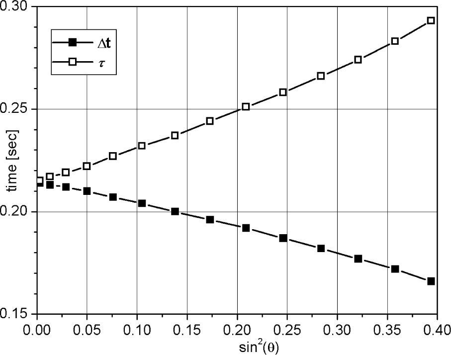
An important value in the calculation of α is the travel time τ of the ray inside the target layer. It is greater than the difference in time between reflected impulses at the same trace, Δt.

A system of non-linear equations can be derived by the tracing method for calculating τ in a multilayered reservoir (Sabinin, 2012). It allows to obtain the difference between Δt and τ, and also the incidence angle θ, and the refraction point x shown in Figure 2.

Figure 2.

Scheme of P-wave reflections in two upper layers of a three-layer medium (the second layer is target).

Alternative methods were developed by Behura & Tsvankin (2009), Shekar & Tsvankin (2011), Reine et al. (2012).

The difference between Δt and τ can be seen in Figure 3. It increases significantly with incidence angle or offset.

Figure 3.

Example of calculating incidence angle θ, travel time τ, and Δt.

As can be seen in Figure 2, one should use the wave reflected from the point x at the top of the target layer to calculate the spectral amplitude A_t (Reine et al., 2012; Sabinin, 2012). This reflected wave can arrive at the surface between receivers. Knowing the value of x, one may obtain this wave (or its spectrum) by interpolation from waves (or spectra) of adjacent traces, taking into account different values of geometrical spreading.

Example of aplication of the techniques

The techniques are compared in ability to give the most precise value of symmetry axis angle ϕ₀ for HTI medium. At present, reliable field methods of obtaining ϕ₀ do not exist. Therefore, I generated synthetic seismograms by applying the technique by Sabinin (2012) of 2D viscoelastic modeling. A three-layer area was constructed with an anisotropic viscoelastic layer in the middle. I set ϕ_{0 =} 60°, and derived models for ϕ_{j =} 0°, 30°, 45°, 75°, 90° by rotating the stiffness tensor for the anisotropic layer.

The stiffness tensor for HTI medium (e.g., Chichinina et al., 2006b) was rotated by 60° to obtain the model for ϕ_{j =} 0°, by 30° for ϕ_{j =} 30°, 90° and by 15° for ϕ_{j =} 45°, 75°. Anisotropic parameters Δ_{N =} 0.35, and Δ_{T =} 0.2 were used in the stiffness tensor.

The attenuation was assumed isotropic in the anisotropic layer, and values of relaxation times were chosen to obtain the factor Q near 60. Host rock velocities V_P in three layers from surface were given the values 3200, 4000, and 4800 m/s, V_S were twice less than V_P; densities were the same for the three layers, and thicknesses of the first two layers from surface were 1590 and 410 m.

A source of explosion type generated one Ricker impulse of frequency 45 Hz. Receivers were spaced over every 200 m beginning from the position of the source, and measured the z-component of velocity.

For data being quasi-real, I added a random Gauss normal (white) noise to the synthetic seismograms generated. Maximum amplitude of the noise was chosen as 10% of the maximum amplitude of the impulse reflected from the top boundary of the target middle layer in the first trace.

In Figure 4, the seismogram for azimuth 0° is presented. As one may see, the amplitude of noise reached up to 50% of the wave amplitude in the middle traces, and up to 100% in far traces.

Figure 4.

Synthetic seismogram with added 10% noise. The x axis is time in ms; the y axis is the number of the trace, each receiver is spaced 200 m. Zero time represents the origin time of the source.

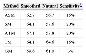
In Table 1, the symmetry axis angles calculated with the proposed numerical methods are compared. The methods were applied both, to traces smoothed by splines of third order and to non-smoothed (natural) traces.

Table 1.

Values of ϕ₀ calculated by different methods.

Method	Smoothed	Natural	Sensitivity^*
ASM	62.7	56.7	15%
SM	64.1	57.6	20%
ATM	57.1	57.8	20%
TM	64.1	64.6	15%
GM	59.6	61.0	3%

*

Sensitivity values are for smoothed traces

For noisy data, the result of estimating ϕ₀ depends on the choice of time windows. The results in Table 1 are obtained with an automatic choice of time windows by a hyperbolic dependence on offset with the initial window set manually. This manual setting was varied up to 10% of the time window.

The results presented in Table 1 are for the best choice of some smart attempts of defining the time windows at the traces. The maximum difference between the estimated ϕ₀ and the correct value of 60° in these attempts, characterizes a sensitivity of the method to the window choice. The approximate values of the sensitivity for smoothed traces are also presented in Table 1.

Discussion and conclusion

The results in Table 1 show superior quality of the General method (GM). It gives stable non-sensitive values with small error. This may be explained by the synthetic nature of the data.

The other methods give good results too, but with a large sensitivity to the choice of time window. For example, 20% for ATM and SM means that one may obtain the value of ϕ₀ with error up to ±12° (0.2x60°).

Smoothing impulses seems to be useful for reducing sensitivity. Smoothing spectra also improves the results.

In synthetic data without noise, all techniques give nearly precise results with low sensitivity.

One can strongly conclude from results for GM that the third term of the approximation in Equation (6) is important when considering synthetic data.

In applying to real field data, the methods can give other results because of other structure of noise.

In real data, the role of the third (squared) term of approximation (6) can become small or wrong. Therefore, the precision of non-truncated methods may be reduced.

The least-squares method used in the techniques gives the better solution, the operating with more traces. Therefore, the methods of sectors (ASM, SM) should give worse results than the others because they operate with much less traces: coarsely k_j≈ n/m.

It should also be noted that SM and ASM are constructed for sectored data and must really on having an additional error because of the need to set a unique value of azimuth for all traces in a sector. This error must be less by decreasing the width of the sector. It must also depend on disposition of the traces inside the sectors.

The maximum value of this error can be easily estimated. For example, let the width of the sector be equal to 10°, and all traces in the sector in the example of previous section be disposed not at the middle azimuth, as above, but at the border of the sector; i.e. at ϕ_j=5°, 35°, 50°, 80°, 95°. This case will consequently correspond to ϕ₀=65°, and to an error of 5° in ϕ₀^.

All suggested methods are not ideal and can be non-reliable in real data. The methods GM, TM, and SM demand the solution of non-linear equations and further choosing one solution from many. This choosing may fail in real data. Contrary, the methods ASM and ATM give only one pair of solutions but use approximate equation (10) instead of (9).

The criterion B_{0 >} 0 for distinguishing the pair of symmetry axis and fracture strike directions, see (7), may unexpectedly fail in real data, too.

The logarithm of spectral ratio may not have the straight linear part near the peaks of the spectra, even in smoothed real data, and therefore the proposed algorithm of setting spectral windows may lead to wrong values of α.

The smoothing by splines is also not the best solution for improving real data.

In such conditions of problems with real data, the best strategy in fracture-reservoir characterization is to apply all these methods together and check if the results obtained with different methods are close to each other. The more methods, the better forecasting.

Here, we discussed some common problems of QVOA techniques. A more careful investigation of the techniques in synthetic data needs to be done in more complicated experiments. The investigation of different methods of smoothing is also interesting. This is a deal of future publications.

Numerical experiments with real data must not use ϕ₀, but other parameters for a comparison of the techniques, because of the correct value ϕ₀ is not known in field data. Such work is beyond the scope of the present publication, and might be hold yet.

Here, the numerical techniques for estimation of fracture directions by applying theory of QVOA analysis were suggested. One of them (GM) is proved good in synthetic data with noise.

Acknowledgement

This work was partially supported by SENER and CONACYT of the Mexican government in the framework of project Y.00108 “Atributos sismicos azimutales de atenuacion y amplitud en datos multicomponentes en el mapeo de fracturas”.