

This paper examines the mutual relationship between banking sector development, insurance sector development, and economic growth in the G-20 countries between 1980 and 2012. Our results demonstrate that there is a long-run equilibrium relationship between these three variables. We then use a panel vector auto-regression model to reveal the nature of Granger causality among these three variables. As expected, we find that both banking sector development and economic growth Granger cause insurance sector development.
A growing literature in financial history has emphasized that the transition to higher and sustained economic growth rates was preceded by the emergence of a modern financial system, sometimes referred to as financial diffusion. The diffusion of well-managed public finances, stable money, a central bank, a banking system, securities markets, and a sound insurance system all play a crucial role in promoting economic development (Andersson, Eriksson, & Lindmark, 2010; Billio, Getmansky, Lo, & Pelizzon, 2012). However, the insurance sector has gained less attention in the finance-growth dilemma (Lee, Lee, & Chiu, 2013; Ward & Zubruegg, 2000).
In this study, we expand the works of Adams, Andersson, Andersson, and Lindmark (2009), Allen and Santomero (2001), Haiss and Sumegi (2008), Horng, Chang, and Wu (2012), Hussels, Ward, and Zurbruegg (2005), Lee (2013) and Liu and Lee (2014) by empirically testing the co-integrating and causal relationship between insurance sector development, banking sector development and economic growth. With the broad use of insurance market in the 1980s, we deploy cross-country panel data to gather enough observations to analyze the causal relationships between the three.
The insurance sector1 has influenced the economy in every aspect (Beck & Webb, 2003; Beenstock, Dickinson, & Khajuria, 1986; Boon, 2005; Chang, Cheng, Pan, & Wu, 2013; Chen, Cheng, Pan, & Wu, 2013; Han, Li, Moshirian, & Tian, 2010; Kugler & Ofoghi, 2005; Lee, 2011; Nektarios, 2010; Outreville, 1996; Pagano, 1993; Sümegi & Haiss, 2008; Wasow & Hill, 1986). The insurance sector contributes to economic growth, both as a financial intermediary and as a provider of risk transfer and indemnification, by allowing different risks to be managed more efficiently and by mobilizing domestic savings (Ward & Zubruegg, 2000). The relationship between insurance sector development2 and economic growth3 has been extensively documented in the financial literature using an array of econometric techniques, such as cross-country, time series, panel data, and firm level studies: for example, Arena (2008), Avram, Nguyen, and Skully (2010), Chang, Cheng, et al. (2013), Chang, Lee, and Chang (2013), Chen, Lee, and Lee (2012), Ching, Kogid, and Furuoka (2010), Curak, Loncar, and Poposki (2009), Enz (2000), Haiss and Sumegi (2008), Han et al. (2010), Lee (2011), Lee and Chiu (2012), Lee, Kwon, and Chung (2010), Lee, Chang, and Chen (2012), Lee, Lee, et al. (2013), Chiu, Tsong, Yang and Chang (2013), Ward and Zubruegg (2000), and Webb, Grace, and Skipper (2005). By and large, the empirical evidence has demonstrated that there is a positive long-run association between the indicators of insurance sector development and economic growth. Many of the papers suggest that a well-developed insurance sector is growth-enhancing, and, therefore, consistent with the proposition of ‘more insurance, more growth’.
This study establishes that insurance sector development has a long-run equilibrium relationship with banking sector development and economic growth. This paper establishes a highly significant positive impact of economic growth and banking sector development on insurance sector development for the G-20 countries, implying that both economic growth and banking sector development play a critical role in boosting insurance sector development in the economies of the G-20.
The rest of the paper is organized as follows. The next section describes the data and the model. The estimation strategy and the empirical results are discussed in “The estimation strategy and empirical results” section. The final section concludes.
Data and modelAnnual data from 1980 to 2012 for the G-20 countries were obtained from the World Development Indicators of the World Bank and Sigma/Economic Research & Consulting, Switzerland. The G-20 consists of 19 member countries plus the European Union (EU), which is represented by the President of the European Council and by the European Central Bank. Although we look at the G-20, within this group of industrialized and developing economies, we observed only 17 member countries, which were used for our analysis.4 The member countries are Argentina, Brazil, China, India, Indonesia, Mexico, the Russian Federation, Saudi Arabia, South Africa, Turkey, Australia, Canada, Italy, Japan, the Korean Republic, the United Kingdom, and the United States.
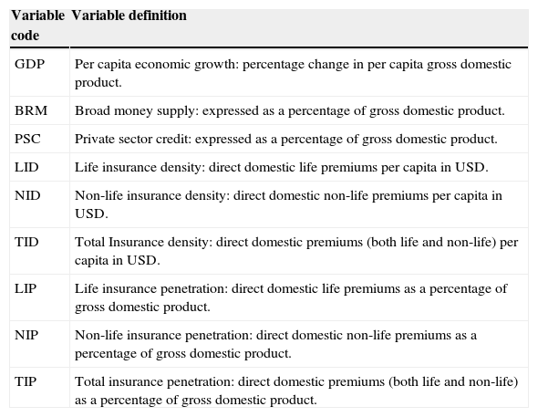
The variables used were the growth rate of real per capita income as a percentage, life insurance5 density as a premium per capita (LID), non-life insurance6 density as a premium per capita (NID), total insurance density as a premium per capita (TID), life insurance penetration as a percentage of gross domestic product (LIP), non-life penetration as a percentage of gross domestic product (NIP), total insurance penetration as a percentage of gross domestic product (TIP), and broad money supply as a percentage of gross domestic product (BRM7). Table 1 presents the detailed discussion of these variables.
Definition of variables.
| Variable code | Variable definition |
|---|---|
| GDP | Per capita economic growth: percentage change in per capita gross domestic product. |
| BRM | Broad money supply: expressed as a percentage of gross domestic product. |
| PSC | Private sector credit: expressed as a percentage of gross domestic product. |
| LID | Life insurance density: direct domestic life premiums per capita in USD. |
| NID | Non-life insurance density: direct domestic non-life premiums per capita in USD. |
| TID | Total Insurance density: direct domestic premiums (both life and non-life) per capita in USD. |
| LIP | Life insurance penetration: direct domestic life premiums as a percentage of gross domestic product. |
| NIP | Non-life insurance penetration: direct domestic non-life premiums as a percentage of gross domestic product. |
| TIP | Total insurance penetration: direct domestic premiums (both life and non-life) as a percentage of gross domestic product. |
Note 1: All monetary measures are in real US dollars.
Note 2: Variables above are defined in the World Development Indicators and published by the World Bank and in World Insurance published by Sigma Economic Research & Consulting, Switzerland.
Note 3: The coverage of these variables is 1988–2012.
Note 4: Insurance penetration, defined as the ratio insurance premium to gross domestic product, associates the scale of the insurance market with that of the economy, but ignores the population factor. On the contrary, insurance density, defined as the premium per capita, takes population into consideration, but neglects economic development.
Note 5: Insurance penetration means direct domestic premiums (for life/non-life/total) in USD expressed as a percentage of gross domestic product.
Note 6: This paper uses these six variables, one at a time, to characterize insurance market development.
Note 7: This paper uses BRM as a representative to banking sector development. However, PSC has also been simultaneously used for some comparative analysis only, particularly in place of BRM.
All three variables were converted into their natural logarithms for estimation purposes.
We used the following model to detect the long-run and short-run causal relationship between insurance sector development (ISD), banking sector development (BSD), and per capita economic growth (GDP).
where, LID, NID, TID, LIP, NIP and TIP are used as proxies for ISD; BRM is used as a proxy for BSD; i=1, 2,…, 17 represent each country in the panel; t=1, 2, …, T (1980–2012) refers to the time period;
The parameters β1ISD and β2ISD represent the long-run elasticity estimates of ISD with respect to GDP and BSD, respectively. The task is to estimate the parameters in Eq. (1) and conduct panel tests on the causal nexus between these three variables. It is postulated that βjISD>0 (for j=1 and 2), which suggests that increases in per capita economic growth (GDP) and banking sector development (BSD) will likely cause an increase in insurance sector development (ISD).
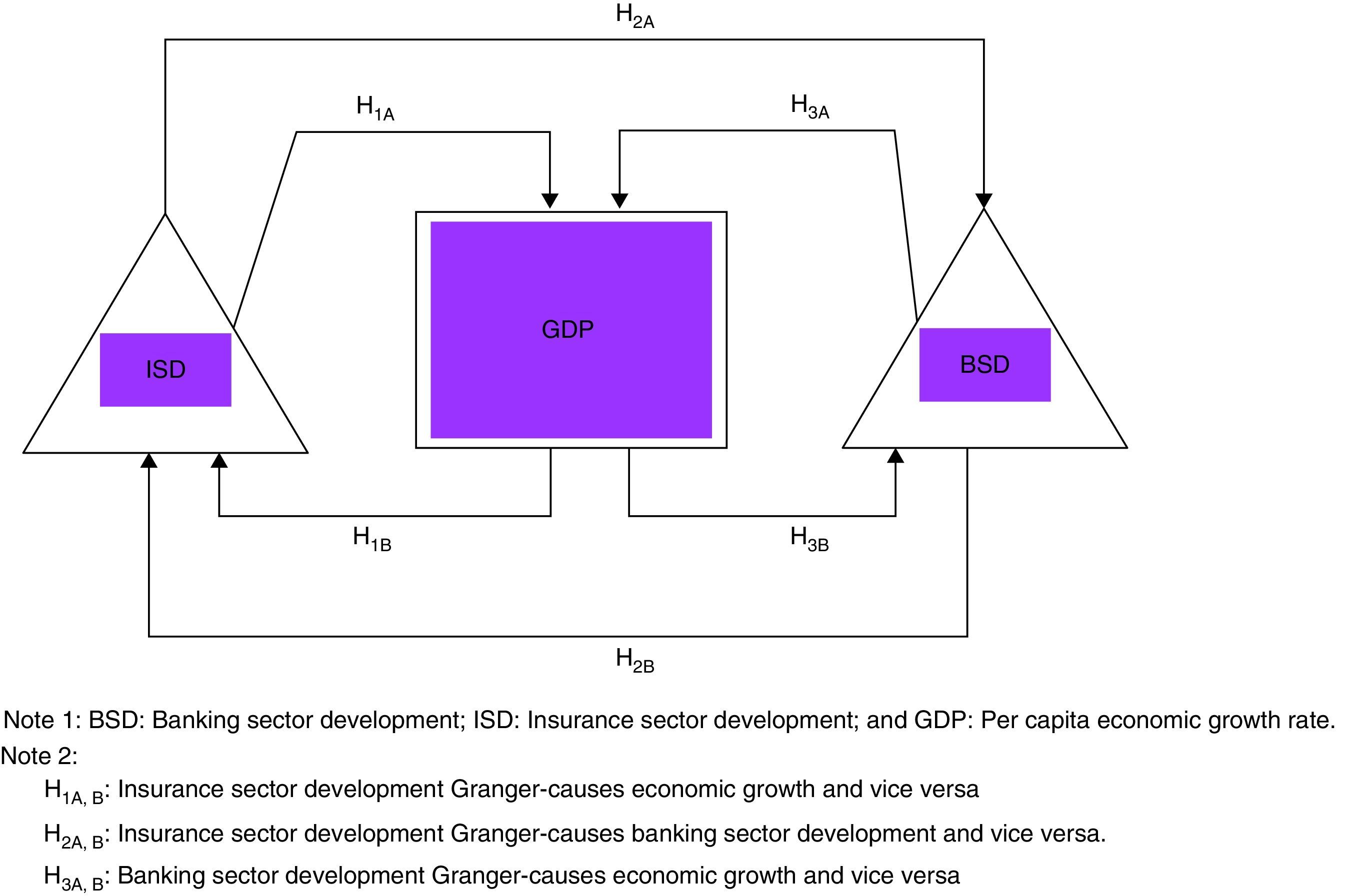
We expect the existence of bidirectional causality between these three variables [ISD–GDP–BSD]. Fig. 1 depicts the bidirectional causal relationship between insurance sector development, banking sector development, and per capita economic growth [H1A, B–H3A, B].
The estimation strategy and empirical results
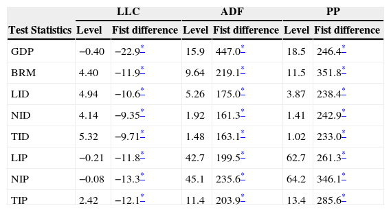
Two types of tests were performed here: a panel cointegration test and a panel Granger causality test. In conducting these tests, the first step of identifying the order of integration at which the variables attain stationarity is essential. Three sets of unit root tests were used for this purpose: the Levin–Lin–Chu (LLC; Levin, Lin, & Chu, 2002), Augmented Dickey Fuller (ADF) and Phillips Perron (PP) panel unit root tests (Choi, 2001). These tests are detailed in several advanced econometric textbooks and are not described here due to space constraints.
Table 2 reports the results of the unit root tests for each variable. Evidently, all of the eight time series variables were non-stationary in their levels. However, they are all stationary at their first difference at the 1% level of significance. In other words, all the variables are integrated of order one (denoted by I (1)) at the individual country and panel levels. Naturally, I (1) meets the requirements of the cointegration test.
Results of panel unit root tests.
| LLC | ADF | PP | ||||
|---|---|---|---|---|---|---|
| Test Statistics | Level | Fist difference | Level | Fist difference | Level | Fist difference |
| GDP | −0.40 | −22.9* | 15.9 | 447.0* | 18.5 | 246.4* |
| BRM | 4.40 | −11.9* | 9.64 | 219.1* | 11.5 | 351.8* |
| LID | 4.94 | −10.6* | 5.26 | 175.0* | 3.87 | 238.4* |
| NID | 4.14 | −9.35* | 1.92 | 161.3* | 1.41 | 242.9* |
| TID | 5.32 | −9.71* | 1.48 | 163.1* | 1.02 | 233.0* |
| LIP | −0.21 | −11.8* | 42.7 | 199.5* | 62.7 | 261.3* |
| NIP | −0.08 | −13.3* | 45.1 | 235.6* | 64.2 | 346.1* |
| TIP | 2.42 | −12.1* | 11.4 | 203.9* | 13.4 | 285.6* |
Note 1: GDP: per capita economic growth rate; BRM: broad money supply; LID: life insurance density; NID: non-life insurance density; TID: total insurance density; LIP: life insurance premium; NIP: non-life insurance premium; TIP: total insurance premium.
* Rejection of the null hypothesis at the 0.01 level.
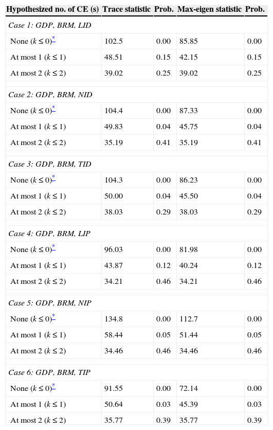
In the subsequent step, we deployed the Johansen cointegration test (Maddala & Wu, 1999), using both trace statistic and maximum eigen values, at the panel setting to check for the existence of cointegration between ISD (LID/NID/TID/LIP/NIP/TIP), BSD and GDP. The discussion of this test is not available here due to space constraints and can be obtainable upon request.
We investigate six different cases by using each insurance sector indicator (LID/NID/TID/LIP/NIP/TIP) separately with BSD and GDP. The results of this test are reported in Table 3. The estimated results indicate that there exists one significant cointegrating vector in each case. It means that our three variables (ISD, BSD and GDP) are linked together by a long-run equilibrium relationship. In other words, we can argue that insurance sector development has a long-run equilibrium relationship with banking sector development and economic growth.
Results of panel cointegration test.
| Hypothesized no. of CE (s) | Trace statistic | Prob. | Max-eigen statistic | Prob. |
|---|---|---|---|---|
| Case 1: GDP, BRM, LID | ||||
| None (k≤0)* | 102.5 | 0.00 | 85.85 | 0.00 |
| At most 1 (k≤1) | 48.51 | 0.15 | 42.15 | 0.15 |
| At most 2 (k≤2) | 39.02 | 0.25 | 39.02 | 0.25 |
| Case 2: GDP, BRM, NID | ||||
| None (k≤0)* | 104.4 | 0.00 | 87.33 | 0.00 |
| At most 1 (k≤1) | 49.83 | 0.04 | 45.75 | 0.04 |
| At most 2 (k≤2) | 35.19 | 0.41 | 35.19 | 0.41 |
| Case 3: GDP, BRM, TID | ||||
| None (k≤0)* | 104.3 | 0.00 | 86.23 | 0.00 |
| At most 1 (k≤1) | 50.00 | 0.04 | 45.50 | 0.04 |
| At most 2 (k≤2) | 38.03 | 0.29 | 38.03 | 0.29 |
| Case 4: GDP, BRM, LIP | ||||
| None (k≤0)* | 96.03 | 0.00 | 81.98 | 0.00 |
| At most 1 (k≤1) | 43.87 | 0.12 | 40.24 | 0.12 |
| At most 2 (k≤2) | 34.21 | 0.46 | 34.21 | 0.46 |
| Case 5: GDP, BRM, NIP | ||||
| None (k≤0)* | 134.8 | 0.00 | 112.7 | 0.00 |
| At most 1 (k≤1) | 58.44 | 0.05 | 51.44 | 0.05 |
| At most 2 (k≤2) | 34.46 | 0.46 | 34.46 | 0.46 |
| Case 6: GDP, BRM, TIP | ||||
| None (k≤0)* | 91.55 | 0.00 | 72.14 | 0.00 |
| At most 1 (k≤1) | 50.64 | 0.03 | 45.39 | 0.03 |
| At most 2 (k≤2) | 35.77 | 0.39 | 35.77 | 0.39 |
Note 1: GDP: per capita economic growth rate; BRM: broad money supply; LID: life insurance density; NID: non-life insurance density; TID: total insurance density; LIP: life insurance premium; NIP: non-life insurance premium; TIP: total insurance premium.
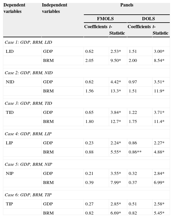
Having confirmed the existence of cointegration of our panel, the next step is to estimate the associated long-run cointegration parameters. Although the ordinary least squares (OLS) estimators of the cointegrated vectors are super-convergent, their distribution is asymptotically biased and depends on nuisance parameters associated with the presence of serial correlation in the data (see, for instance, Pedroni, 2001). Many types of problems existing in the time series analysis may also arise for the panel data analysis and tend to be more marked, even in the presence of heterogeneity (Kao and Chiang, 2001). For this reason, several estimators have been proposed. The study uses two panel cointegration estimators: the between group fully modified OLS (FMOLS8) and dynamic OLS (DOLS9). Both FMOLS and DOLS provide consistent estimates of standard errors that can be used for inference. According to Kao and Chiang (2000), both FMOLS and DOLS estimators have normal limiting properties. The models start with the estimation of the following regression equation.
where, Yit represents log ISD and Xit represents log GDP and log BSD. Both Yit and Xit are cointegrated with slopes βi, which may or may not be homogenous across i.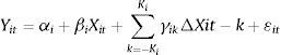
Following Eq. (2), let ξit=εˆitΔXit be a stationary vector consisting of the estimated residuals from the cointegrating regression.
Also let Ωit=lim T→∞T−1∑t=1Tξit∑t=1Tξit′ be the long-run covariance for this vector process which can be decomposed into Ωit=Ωit0+Γi+Γ′i, where Ωit0 is the contemporaneous covariance and Γii is a weighted sum of autocovariances.
Thus, the panel FMOLS estimator will be given by
where Yit*=(Yit−Y¯)−(Ωˆ21i/Ωˆ22i)ΔXit and γˆi=Γˆ21i+Γˆ21i0−(Ωˆ21i/Ωˆ22i)(Tˆ22i/Ωˆ22i0)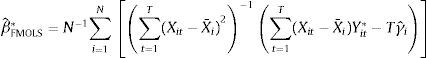
On the contrary, with the DOLS approach, as developed by Kao and Chiang (2001) and Mark and Sul (2003), the concerning estimator is coming from Eq. (2) which includes advanced and delayed values (ΔXiT) in the cointegrated relationship, in order to eliminate the correlation between the regressor and the error terms. Hence the panel DOLS estimator can be defined as
where, Zit=[Xit−X¯,ΔXit−ki,....ΔXt+Ki] is the vector of the regressor, and Yˆit=[Yit−Y¯].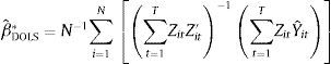
To carry out tests on the cointegrated vectors, it is consequently necessary to use methods of effective estimation.
The results of this section are presented in Table 4.
Panel FMOLS and DOLS results.
| Dependent variables | Independent variables | Panels | |||
|---|---|---|---|---|---|
| FMOLS | DOLS | ||||
| Coefficients | t-Statistic | Coefficients | t-Statistic | ||
| Case 1: GDP, BRM, LID | |||||
| LID | GDP | 0.62 | 2.53* | 1.51 | 3.00* |
| BRM | 2.05 | 9.50* | 2.00 | 8.54* | |
| Case 2: GDP, BRM, NID | |||||
| NID | GDP | 0.62 | 4.42* | 0.97 | 3.51* |
| BRM | 1.56 | 13.3* | 1.51 | 11.9* | |
| Case 3: GDP, BRM, TID | |||||
| TID | GDP | 0.65 | 3.84* | 1.22 | 3.71* |
| BRM | 1.80 | 12.7* | 1.75 | 11.4* | |
| Case 4: GDP, BRM, LIP | |||||
| LIP | GDP | 0.23 | 2.24* | 0.86 | 2.27* |
| BRM | 0.88 | 5.55* | 0.86** | 4.88* | |
| Case 5: GDP, BRM, NIP | |||||
| NIP | GDP | 0.21 | 3.55* | 0.32 | 2.84* |
| BRM | 0.39 | 7.99* | 0.37 | 6.99* | |
| Case 6: GDP, BRM, TIP | |||||
| TIP | GDP | 0.27 | 2.85* | 0.51 | 2.58* |
| BRM | 0.82 | 6.69* | 0.82 | 5.45* | |
Note 1: GDP: per capita economic growth rate; BRM: broad money supply; LID: life insurance density; NID: non-life insurance density; TID: total insurance density; LIP: life insurance premium; NIP: non-life insurance premium; TIP: total insurance premium.
Note 2: * and ** denote rejection of the null hypothesis at the 0.01 and 0.05 levels.
We are mostly interested in knowing the nature of the relationship, be it positive or negative, of the variables. It can be seen that both GDP and BSD exercise a significant positive influence on ISD in the long-run. The finding of the presence of a highly significant positive impact of economic growth and banking sector development on insurance sector development for the G-20 countries implies that both economic growth and banking sector development play a critical role in boosting insurance sector development in the economies of the G-20. For instance, the panel long-run growth elasticity is 0.62 in Case 1 (see Table 4, row 1 and column 1). This implies that a 1% increase in economic growth can increase insurance market development by 0.62%. This is exactly the same in Case 2 and 0.65%, 0.23%, 0.21% and 0.27% in Cases 3–6. Similarly, a 1% increase in banking sector development can increase the insurance market development by 0.39–2.05%, in all the occasions (Cases 1–6; Table 4).
Engle and Granger (1987) demonstrated that when variables are cointegrated, an error correction model necessarily describes the data-generating process. Therefore, on the basis of the unit root and cointegration test results above, the vector error-correction models, VECMs, were used to determine the causal relations between the variables. In other words, we sought to determine what variable caused the other in the presence of the third variable. We were able to determine this causal link for both the short-run and the long-run. Following the Arellano and Bond (1991) and Holtz-Eakin, Newey, and Rosen (1988) estimation procedures, we deployed the following VECMs to trace the causal links between insurance development, banking sector development and economic growth.
where, Δ is the first difference operator; i represents the country in the panel (i=1, 2, …, N); t denotes the year in the panel (t=1, 2, …., T); p, q, and r are lag lengths for the differenced variables of the respective equations and can be determined by the Engle–Granger approach;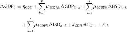
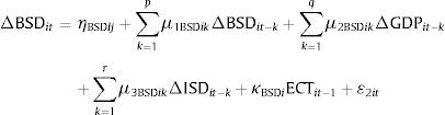
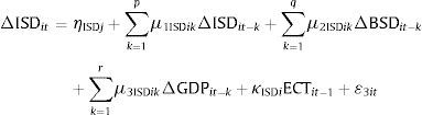
The subscript ‘i’ was removed from the equation when we conducted individual country analysis; ¿it is a normally distributed random error term for all i and t with a zero mean and a finite heterogeneous variance;
The ECTs are error-correction terms, derived from the cointegrating equations. The ECTs represent the long-run dynamics, while differenced variables represent the short-run dynamics between the variables. Put differently, ECTs indicate the extent of the deviation from the long-run equilibrium which was present in the previous period. The coefficients of ECT fulfill the role of the adjustment parameter, which show the proportion of the disequilibrium that is recovered during the subsequent period. On the contrary, the coefficients of the lagged-first differences provide an indication of the short-run relationship between the endogenous variables (Harris & Sollis, 2006; Enders, 2004).
For short-run causal relationships, if the null hypothesis of μ2GDP=0 in Eq. (5) (or μ2BSD=0 in Eq. (6)) is rejected, this implies that there is Granger causality running from BSD to GDP, or from GDP to BSD. Similarly, if the joint null hypothesis of μ3GDP=0 in Eq. (5) (or μ3ISD=0 in Eq. (7)) is rejected, then Granger causality is running from ISD to GDP, or from GDP to ISD. Again, if the joint null hypothesis of μ3BSD=0 in Eq. (6) (or μ2ISD=0 in Eq. (7)) is rejected, then Granger causality is running from ISD to BSD, or from BSD to ISD. We use both Akaike Information Criterion and Schwarz Information Criterion to determine the optimal lag lengths of the VECMs.
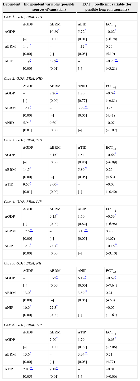
For long-run causal relationships, the null hypothesis (κGDP=0, κBSD=0, and κISD=0) needed to be rejected. The above tests can be achieved via a Wald test. The results of the Granger causality test are shown in Tables 5 and 6. Table 5 reports both short-run and long-run causality, based on the significance of the lagged ECT coefficients, while Table 6 reports the summary of short-run causality, based on the significance of Wald-statistics.
Results of panel granger causality test.
| Dependent | Independent variables (possible sources of causation) | ECT−1 coefficient variable (for possible long run causality) | ||
|---|---|---|---|---|
| Case 1: GDP, BRM, LID | ||||
| ΔGDP | ΔBRM | ΔLID | ECT−1 | |
| ΔGDP | – | 10.89* | 5.72* | −0.62* |
| [–] | [0.00] | [0.01] | (−6.78) | |
| ΔBRM | 14.4* | – | 4.12** | 0.25 |
| [0.00] | [–] | [0.05] | (5.19) | |
| ΔLID | 11.9* | 5.69* | – | −0.23** |
| [0.00] | [0.01] | [–] | (−3.21) | |
| Case 2: GDP, BRM, NID | ||||
| ΔGDP | ΔBRM | ΔNID | ECT−1 | |
| ΔGDP | – | 8.26* | 1.80 | −074* |
| [–] | [0.00] | [0.77] | (−6.81) | |
| ΔBRM | 12.1* | – | 3.99** | 0.25 |
| [0.00] | [–] | [0.05] | (4.41) | |
| ΔNID | 5.94* | 9.60* | – | −0.07 |
| [0.01] | [0.00] | [–] | (−1.07) | |
| Case 3: GDP, BRM, TID | ||||
| ΔGDP | ΔBRM | ΔTID | ECT−1 | |
| ΔGDP | – | 8.15* | 1.54 | −0.66* |
| [–] | [0.00] | [0.80] | (−6.09) | |
| ΔBRM | 14.5* | – | 5.80** | 0.26 |
| [0.00] | [–] | [0.05] | (4.63) | |
| ΔTID | 9.57* | 9.60* | – | −0.03 |
| [0.01] | [0.00] | [–] | (−0.40) | |
| Case 4: GDP, BRM, LIP | ||||
| ΔGDP | ΔBRM | ΔLIP | ECT−1 | |
| ΔGDP | – | 9.15* | 1.50 | −0.59* |
| [–] | [0.00] | [0.82] | (−6.98) | |
| ΔBRM | 12.6** | – | 3.16** | 0.20 |
| [0.00] | [–] | [0.05] | (4.67) | |
| ΔLIP | 12.3* | 7.07* | – | −0.16** |
| [0.00] | [0.00] | [–] | (−3.10) | |
| Case 5: GDP, BRM, NIP | ||||
| ΔGDP | ΔBRM | ΔNIP | ECT−1 | |
| ΔGDP | – | 8.72* | 6.12* | −0.69* |
| [–] | [0.00] | [0.00] | (−7.64) | |
| ΔBRM | 13.0* | – | 3.89** | 0.21 |
| [0.00] | [–] | [0.05] | (4.53) | |
| ΔNIP | 16.6* | 22.3* | – | −0.05 |
| [0.00] | [0.00] | [–] | (−1.67) | |
| Case 6: GDP, BRM, TIP | ||||
| ΔGDP | ΔBRM | ΔTIP | ECT−1 | |
| ΔGDP | – | 7.20* | 1.79 | −0.63* |
| [–] | [0.00] | [0.77] | (−7.06) | |
| ΔBRM | 13.6* | – | 3.94** | 0.21 |
| [0.00] | [–] | [0.05] | (4.77) | |
| ΔTIP | 2.87** | 9.18* | – | −0.01 |
| [0.05] | [0.01] | [–] | (−0.06) | |
Note 1: GDP: per capita economic growth rate; BRM: broad money supply; LID: life insurance density; NID: non-life insurance density; TID: total insurance density; LIP: life insurance premium; NIP: non-life insurance premium; TIP: total insurance premium.
Note 2: VECM: vector error correction model; ECT: error correction term.
Note 3: Values in squared brackets represent probabilities for F-statistics.
Note 4: Values in parentheses represent t-statistics.
Note 5: Basis for the determination of long run causality lies in the significance of the lagged ECT coefficient.
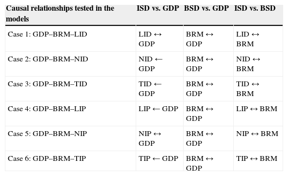
The summary of short-run granger causality.
| Causal relationships tested in the models | ISD vs. GDP | BSD vs. GDP | ISD vs. BSD |
|---|---|---|---|
| Case 1: GDP–BRM–LID | LID↔GDP | BRM↔GDP | LID↔BRM |
| Case 2: GDP–BRM–NID | NID←GDP | BRM↔GDP | NID↔BRM |
| Case 3: GDP–BRM–TID | TID←GDP | BRM↔GDP | TID↔BRM |
| Case 4: GDP–BRM–LIP | LIP←GDP | BRM↔GDP | LIP↔BRM |
| Case 5: GDP–BRM–NIP | NIP↔GDP | BRM↔GDP | NIP↔BRM |
| Case 6: GDP–BRM–TIP | TIP←GDP | BRM↔GDP | TIP↔BRM |
Note 1: GDP: per capita economic growth rate; BRM: broad money supply; LID: life insurance density; NID: non-life insurance density; TID: total insurance density; LIP: life insurance premium; NIP: non-life insurance premium; TIP: total insurance premium.
Note 2: X→Y means variable X Granger causes variable Y; X←Y means variable Y Granger causes X; and X↔Y means both variables Granger cause each other; NA: no causality happening between the two variables.
From Table 5, when we considered ΔGDP as the dependent variable, we found the existence of long-run causal relationships between economic growth, insurance sector development and banking sector development. The estimated lagged ECTs (Cases 1–6) all carry negative signs, as expected. This implies that the change in the level of economic growth (ΔGDP) rapidly responds to any deviation in the long-run equilibrium (or short-run disequilibrium) for the t−1 period. In other words, the effect of an instantaneous shock to insurance market development and banking sector development on economic growth will be completely adjusted in the long-run. The return to equilibrium, however, occurs at different rates: 62% in Case 1, 74% in Case 2, 66% in Case 3, 59% in Case 4, 69% in Case 5, and 63% in Case 6.
The long-run causal relationships between economic growth, insurance sector development and banking sector development also exist when ΔLID and ΔLIP were used as the dependent variables. The speeds of adjustment for these two cases are 23% and 16% for Case 1 and Case 4, respectively. However, when we considered ΔBSD or ΔISD (for ΔNID, ΔTID, ΔNIP and ΔTIP) as the dependent variable, we found non-uniform results. That means the ECTs are not statically significant. The statistical insignificance of the ECTs suggests that economic growth (or BSD or ISD) does not respond to deviations from long-run equilibrium.
From these results, the common insight is that both insurance sector development and banking sector development drive economic growth in the G-20 countries.
In contrast to the long-run Granger causality results, our study reveals a wide spectrum of short-run causality results between the three variables (ISD, BSD and GDP). These results are summarized in Table 6 and are presented below.
In Case 1, we find the existence of bidirectional causality between broad money supply and economic growth [BRM↔GDP], life insurance density and economic growth [LID↔GDP], and between life insurance density and broad money supply [LID↔BRM]. This gives the evidence of two-way Granger causality (feedback) between BRM and GDP, LID and GDP, and LID and BRM. That means there is support for both the supply-leading10 hypothesis and the demand-following11 hypothesis. The inference, particularly for the LID–GDP nexus, is that insurance sector development and economic growth are endogenous. This indicates that they mutually cause each other and that their reinforcement may have important implications for the development of financial and economic policies.
In Case 2, we find the existence of bidirectional causality between broad money supply and economic growth [BRM↔GDP] and non-life insurance density and broad money supply [NID↔BRM]. Furthermore, we find the unidirectional causality from economic growth to non-life insurance density [GDP→NID]. This supports the feedback relationship between banking sector development and economic growth as well as between banking sector development and insurance sector development. In addition, it supports the demand-following hypothesis between insurance sector development and economic growth, implying that as real per capita growth increases, investors and savers will require various new financial services, thus leading to the creation of modern financial institutions and related financial services.
In Case 3, we establish the presence of bidirectional causality between broad money supply and economic growth [BRM↔GDP] and total insurance density and broad money supply [TID↔BRM]. Moreover, we find the unidirectional causality from economic growth to total insurance density [GDP→TID]. These results are very similar to those of Case 2 [NID–GDP–BRM].
In Case 4, we detect the continuation of bidirectional causality between broad money supply and economic growth [BRM↔GDP] and life insurance penetration and broad money supply [LIP↔BRM]. In addition, we find unidirectional causality from economic growth to life insurance penetration [GDP→LIP]. These results are very similar to those of Case 2 [NID–GDP–BRM] and Case 3 [TID–GDP–BRM].
In Case 5, we come across the presence of bidirectional causality between broad money supply and economic growth [BRM↔GDP], non-life insurance penetration and economic growth [NIP↔GDP], and between non-life insurance penetration and broad money supply [NIP↔BRM]. These results are very similar to Case 1 [LID–GDP–BRM].
In Case 6, we find the existence of bidirectional causality between broad money supply and economic growth [BRM↔GDP] and total insurance penetration and broad money supply [TIP↔BRM]. Furthermore, we find unidirectional causality from economic growth to total insurance penetration [GDP→TIP]. These results are very similar to Case 2 [NID–GDP–BRM], Case 3 [TID–GDP–BRM] and Case 4 [LIP–GDP–BRM].
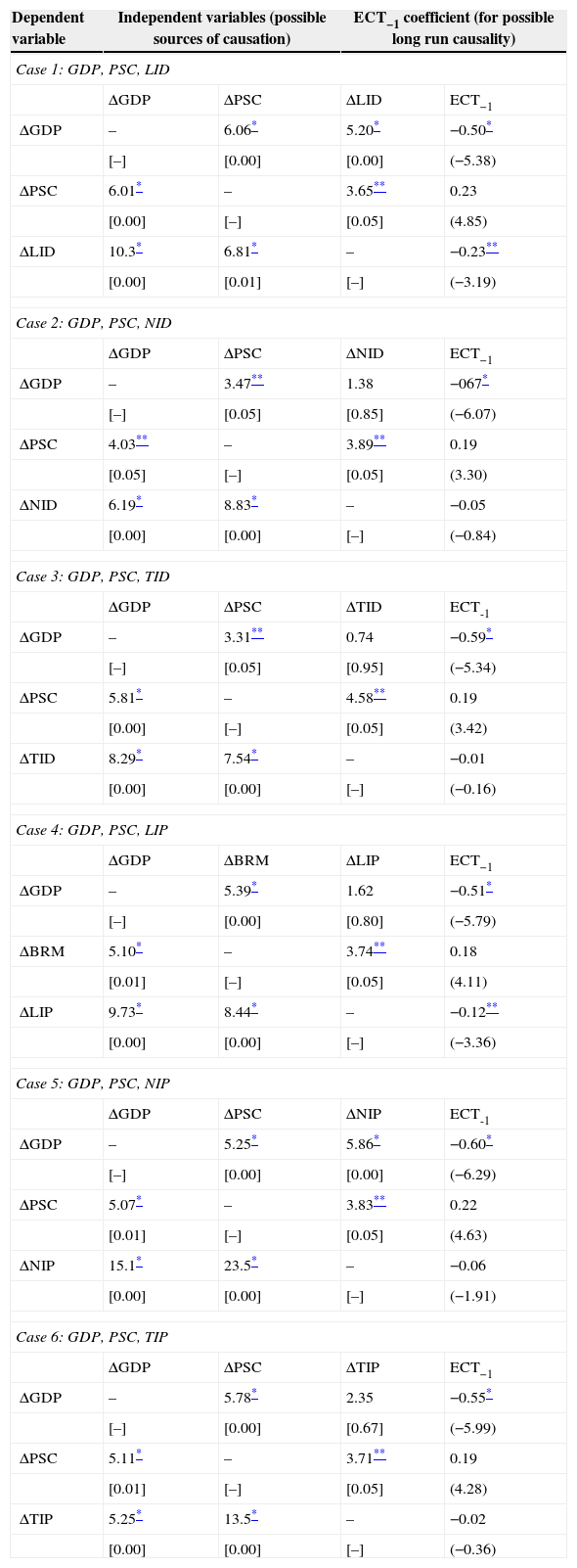
The above discussion, as per Arellano and Bond (1991) and Holtz-Eakin et al. (1988) estimation procedures, is one way of checking the direction of Granger causality between insurance sector development, banking sector development and economic growth. Nonetheless, this estimation procedure does not provide much information on how each variable responds to innovations in other variables, or whether the shock is permanent or not. To avoid this shortcoming, we employ generalized impulse response functions (GIRFs), developed by Koop, Pesaran, and Potter (1996), to trace the effect of a one-off shock to one of the innovations on the current and future values of the endogenous variables. The GIRFs offer additional insight into how shocks to insurance development can affect and be affected by each of the other two variables: economic growth and banking sector development. These results are not available here due to space constraints but can be obtained upon request. Furthermore, we have also tested the results between economic growth, insurance sector development and banking sector development, where we replace private sector credit with broad money supply. The findings are almost similar, like the case of the inclusion of broad money supply. We just report the Granger causality results of this portion in the Appendix A.
Even though the majority of the results12 are similar, still some minor differences exist, particularly between insurance sector development and economic growth. In general, it is worthwhile to note that our panel short-run Granger causality results seem to be in line with some of the previous studies. For instance, the findings of bidirectional Granger causality between banking sector development and economic growth is well supported by the findings of Pradhan, Arvin, Norman and Hall (2014), Pradhan, Arvin, Norman, and Nishigaki (2014),13Wolde-Rufael (2009),14Craigwell, Downes, and Howard (2001),15 and Ahmed and Ansari (1998).16 The results of bidirectional Granger causality between banking sector development and insurance sector development are in line with Liu and Lee (2014),17 and Vadlamannati (2008).18 The finding of unidirectional Granger causality from economic growth to insurance sector development is well supported by the findings of Horng et al. (2012),19 and Vadlamannati (2008). Furthermore, the finding of bidirectional Granger causality economic growth and insurance sector development is in line with the findings of Chang, Cheng, et al. (2013), Chang, Lee, et al. (2013),20Vadlamannati (2008), and Ward and Zubruegg (2000).21
ConclusionThe financial system has become noticeably more complex over the past couple of decades as the separation between hedge funds, mutual funds, insurance companies, banks, and brokers/dealers has blurred thanks to financial diffusion and deregulation. While such complexities are an unavoidable consequence of competition and economic growth, it is accompanied by certain advantages, including much greater interdependence (Billio et al., 2012).
This paper investigates the interdependence between insurance market development, banking sector development, and economic growth. Using panel data relating to G-20 countries from 1988 to 2012, we find that both banking sector development and economic growth exercise a significant positive effect on insurance sector development. The study additionally finds that insurance market development, banking sector development, and economic growth are cointegrated. The panel Granger causality tests further confirm that both banking sector development and economic growth Granger-cause insurance sector development in the long run. However, in the short-run, we detect the bidirectional causality between banking sector development and economic growth and between banking sector development and insurance sector development. We also notice economic growth Granger causes insurance sector development, particularly for non-life insurance density, total insurance density, life insurance premium and total insurance premium. However, for life insurance density and non-life insurance premium, they reinforce each other, e.g., the existence of a feedback relationship between economic growth and insurance sector development.
The main message from this study for policy-makers is that inferences drawn from research on economic growth that excludes the dynamic interrelation between insurance sector development and banking sector development may be unreliable. Policymakers need to eagerly reform the financial system in these G-20 countries in order to strengthen the cooperative relationship between the insurance sector and the banking sector and achieve their interactive effects on economic growth.
Following the results of this empirical investigation, the implication of studies of this sort is that, a policy framework aimed at increasing banking sector development and economic growth might help increase insurance sector development. The development of the insurance sector can also be utilized properly for obtaining more banking sector development and achieving sustainable economic growth in the G-20 countries. For instance, an active and competitive insurance sector can enable these economies in stimulating savings, catering an alternate source of investment, reinforcing the development of the stock market and bond market, mitigating risks associated to volatility in capital inflows, and can shift government burden in supporting large pension schemes to employee insurance-supported retirement schemes.
The important requirement is that the government of these respective countries should encourage financial products innovation and the diffusion of combining insurance markets with the banking sector, in order to promote collaborative developments of both the insurance and the banking sector. Furthermore, for achieving sustainable economic growth, it is advantageous to bring more reform in both the insurance sector and the banking sector in order to improve information flow, better service delivery and to enhance competition. It is the conjoint interaction between these variables that distinguishes our study and guides future research on this topic.
We thank the Editor and an anonymous referee for their comments and suggestions.
See Table A1.
Results of panel granger causality test (by replacing BRM with PSC).
| Dependent variable | Independent variables (possible sources of causation) | ECT−1 coefficient (for possible long run causality) | ||
|---|---|---|---|---|
| Case 1: GDP, PSC, LID | ||||
| ΔGDP | ΔPSC | ΔLID | ECT−1 | |
| ΔGDP | – | 6.06* | 5.20* | −0.50* |
| [–] | [0.00] | [0.00] | (−5.38) | |
| ΔPSC | 6.01* | – | 3.65** | 0.23 |
| [0.00] | [–] | [0.05] | (4.85) | |
| ΔLID | 10.3* | 6.81* | – | −0.23** |
| [0.00] | [0.01] | [–] | (−3.19) | |
| Case 2: GDP, PSC, NID | ||||
| ΔGDP | ΔPSC | ΔNID | ECT−1 | |
| ΔGDP | – | 3.47** | 1.38 | −067* |
| [–] | [0.05] | [0.85] | (−6.07) | |
| ΔPSC | 4.03** | – | 3.89** | 0.19 |
| [0.05] | [–] | [0.05] | (3.30) | |
| ΔNID | 6.19* | 8.83* | – | −0.05 |
| [0.00] | [0.00] | [–] | (−0.84) | |
| Case 3: GDP, PSC, TID | ||||
| ΔGDP | ΔPSC | ΔTID | ECT-1 | |
| ΔGDP | – | 3.31** | 0.74 | −0.59* |
| [–] | [0.05] | [0.95] | (−5.34) | |
| ΔPSC | 5.81* | – | 4.58** | 0.19 |
| [0.00] | [–] | [0.05] | (3.42) | |
| ΔTID | 8.29* | 7.54* | – | −0.01 |
| [0.00] | [0.00] | [–] | (−0.16) | |
| Case 4: GDP, PSC, LIP | ||||
| ΔGDP | ΔBRM | ΔLIP | ECT−1 | |
| ΔGDP | – | 5.39* | 1.62 | −0.51* |
| [–] | [0.00] | [0.80] | (−5.79) | |
| ΔBRM | 5.10* | – | 3.74** | 0.18 |
| [0.01] | [–] | [0.05] | (4.11) | |
| ΔLIP | 9.73* | 8.44* | – | −0.12** |
| [0.00] | [0.00] | [–] | (−3.36) | |
| Case 5: GDP, PSC, NIP | ||||
| ΔGDP | ΔPSC | ΔNIP | ECT-1 | |
| ΔGDP | – | 5.25* | 5.86* | −0.60* |
| [–] | [0.00] | [0.00] | (−6.29) | |
| ΔPSC | 5.07* | – | 3.83** | 0.22 |
| [0.01] | [–] | [0.05] | (4.63) | |
| ΔNIP | 15.1* | 23.5* | – | −0.06 |
| [0.00] | [0.00] | [–] | (−1.91) | |
| Case 6: GDP, PSC, TIP | ||||
| ΔGDP | ΔPSC | ΔTIP | ECT−1 | |
| ΔGDP | – | 5.78* | 2.35 | −0.55* |
| [–] | [0.00] | [0.67] | (−5.99) | |
| ΔPSC | 5.11* | – | 3.71** | 0.19 |
| [0.01] | [–] | [0.05] | (4.28) | |
| ΔTIP | 5.25* | 13.5* | – | −0.02 |
| [0.00] | [0.00] | [–] | (−0.36) | |
Note 1: GDP: per capita economic growth rate; BRM: broad money supply; PSC: private sector credit; LID: life insurance density; NID: non-life insurance density; TID: total insurance density; LIP: life insurance premium; NIP: non-life insurance premium; TIP: total insurance premium.
Note 2: VECM: vector error correction model; ECT: error correction term.
Note 3: Values in squared brackets represent probabilities for F-statistics.
Note 4: Values in parentheses represent t-statistics.
Note 5: Basis for the determination of long run causality lies in the significance of the lagged ECT coefficient.
Insurance, like other financial services, has grown in quantitative importance as part of the general development of financial institutions. The governments of many developing countries have historically held the view that the financial systems they inherited could not adequately serve their countries’ developmental needs. Therefore, during the past several years, they have directed considerable efforts toward changing the structure of these financial systems and controlling their operations in order to channel savings to investments, which are crucial components of development programs (Outreville, 1990; UNCTD, 1988).
Insurance market development refers to a process that marks improvements in the quantity, quality and efficiency of the insurance sector.
The broad literature focusing on the various determinants of economic growth is not surveyed here. See, for example, Barro and Sala-i-Martin (1995).
To include the EU, the twentieth member, would have meant double-counting four countries: France, Germany, Italy, and the United Kingdom. However, later we exclude both France and Germany due to the non-availability of data for broad money supply.
Life insurance, in its general form, is guaranteed to pay a specific amount of indemnification to a beneficiary after the insured's death or to the insured who lives beyond a certain age.
In contrast to life insurance, non-life insurance includes all other types of insurance, such as homeowner's insurance, motor vehicle insurance, marine insurance, liability insurance, etc. (Chen et al., 2013).
BRM, as a representative to banking sector development, is a cardinal to foster long-run economic growth. There are many channels through which BRM (or private sector credit, another banking sector development indicator) can contribute to long-run economic growth. These channels are (a) rendering information about possible investments, so as to allocate capital efficiently; (b) supervising firms and exerting corporate governance; (c) diversifying risk; (d) mobilizing and pooling savings; (e) facilitating the exchange of goods and services; and (f) easing technology transfer (see, for instance, Pradhan, Arvin, Norman & Hall, 2014).
FMOLS is a non-parametric approach, taking into account the possible correlation between the error term and the first differences of the regressor as well as the presence of a constant term to deal with corrections for serial correlation (see, for instance, Maeso-Fernandez et al., 2006; Pedroni, 2000, 2001).
DOLS is a parametric approach, which adjusts the errors by augmenting the static regression with leads, lags, and contemporaneous values of the regressor in first differences (see, for instance, Kao & Chiang, 2000).
The supply-leading hypothesis, for the finance-growth nexus, implies more financial services (banking/insurance) leads to more economic growth.
The demand-following hypothesis implies more economic growth leads to an increase in the demand for financial services.
The definition of the variables is not always uniform across the studies.
The study dealt with 26 ASEAN Regional Forum countries for the period 1961–2012.
The study was in Kenya for the period 1966–2005.
The study was in Barbados for the period 1974–1998.
The study dealt with three Asian countries: India, Pakistan and Sri Lanka for the period 1973–1991.
The study was in China for the period 1985–2011.
The study was in India for the period 1980–2006.
The study was in Taiwan for the period 1961–2006.
The study dealt with eight Eastern Asian countries, namely India, Indonesia, Japan, Malaysia, the Philippines, Singapore, South Korea, and Thailand, for the period 1979–2008.
The study included nine OECD countries, namely Australia, Austria, Canada, France, Italy, Japan, Switzerland, the United Kingdom, and the United States, for the period 1961–1996.

www.publicationethics.org.