


The empirical tests of traditional structural models of credit risk tend to indicate that such models have been unsuccessful in the modeling of credit spreads. To address these negative findings some authors introduce single-factor stochastic volatility specifications and/or jumps.
In the yield curve literature it is widely accepted that one-factor is not sufficient to capture the time variation and cross-sectional variation in the term structure. This article introduces a two-factor stochastic volatility specification within the structural model of credit risk. One of the factors determines the correlation between short-term firms’ assets returns and variance, whereas the other factor determines the correlation between long-term returns and variance. The numerical tests reveal how the introduction of two volatility factors can generate a wide range of combinations associated with short-term and long-term patters corresponding to credit spreads. In this sense, multi-factor stochastic volatility specifications provide more flexibility than single-factor models to capture a wide range of shapes associated with the term structure of credit spreads consistent with the empirical evidence.
Structural models of credit risk formulate explicit assumptions about the dynamics of a firm's assets, its capital structure and its debt. In this case, the default event happens if firm's assets are not sufficient to pay the debt and corporate liabilities can be considered as contingent claims on the firm's assets. The credit risk literature based on the structural approach begins with the study of Merton (1974), who applies the option pricing theory developed by Black and Scholes (1973) to model credit spreads, where the credit spread is defined as the difference between the yield of a corporate bond and the associated yield on Treasury bonds with the closest matching maturity.
The empirical tests of traditional structural models of credit risk tend to indicate that such models have been unsuccessful in the modeling of credit spreads. In particular, Jones et al. (1984) and Huang and Huang (2003), among others, show that predicted credit spreads are far below observed ones. To address these negative findings some authors, such as Zhang et al. (2009), introduce a single-factor stochastic volatility model with jumps within the Merton (1974) framework. They show that their model improves the match between predicted and observed credit spreads, especially for investment-grade companies. Unfortunately, the results are less satisfactory for low investment grade and speculative grade. In theory, jumps can help to match the observed credit spread levels for investment grade bonds and short maturities. But empirical evidence is rather inconclusive. Collin-Dufresne et al. (2003) have found that only a small fraction of observed credit spreads of aggregate portfolios can be explained by jump risk. On the other hand, Cremers et al. (2008) suggest that the addition of jumps and jump risk premia brings predicted yield spread levels much closer to observed ones.
Importantly, the study of Zhang et al. (2009) considers a single stochastic volatility factor as in Heston (1993). Within the equity option valuation context, Christoffersen et al. (2009) extend the original Heston (1993) framework to generate a two-factor stochastic volatility model built upon the square root process. This article introduces a two-factor stochastic volatility specification within the structural Merton (1974) framework. The advantage is that a two-factor model provides more flexibility to model the volatility term structure. In this sense, one of the factors determines the correlation between short-term firms’ assets returns and variance, whereas the other factor determines the correlation between long-term returns and variance. Hence, the two-factor specification is able to generate more flexible credit spread term structures to match the observed term structures associated with credit spreads.
The rest of the paper proceeds as follows. Section 2 presents the main features of the two-factor stochastic volatility specification and develops semi-closed-form solutions for the price of credit spreads and default probabilities. Section 3 provides a numerical analysis which shows that the model is able to generate credit spread term structures consistent with the empirical evidence. This section also offers a sensitivity analysis of credit spreads with respect to the model parameters. Finally, Section 4 offers concluding remarks.
2A structural model of credit risk under a two-factor stochastic volatility frameworkLet us assume the same market framework as in Merton (1974). Within this framework, firms issue a zero coupon bond with a promised payment B at maturity t=T. In this case, default occurs only at maturity with debt face value as default boundary. In the event of default, the absolute priority rule prevails.
Let At∈ℝt≥0 be the price process of the firm's assets and let us denote by Yt=lnAt the log-return vector. For simplicity, I assume that the continuously compounded risk-free rate r and asset payout ratio q are constant. Let Θ denote the probability measure defined on a probability space Λ,Ϝ,Θ such that asset prices expressed in terms of the current account are martingales. We denote this probability measure as the risk-neutral measure. As in Christoffersen et al. (2009), I consider a two-factor specification for the variance process and I assume the following dynamics for the return process Yt under Θ:
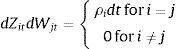
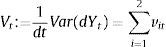
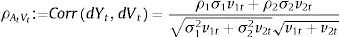
with:where θi represents the long-term mean corresponding to the instantaneous variance factor i (for i=1, 2), κi denotes the speed of mean reversion and, finally, σi represents the volatility of the variance factor i. For analytical convenience, let us rewrite the previous equation as follows:where bi=κi and ai=κiθi. In Eqs. (1) and (2)Zit and Wit are Wiener processes such that:On the other hand, Z1t and Z2t are uncorrelated. In addition, W1t and W2t are also uncorrelated. The single-factor Heston (1993) model can be obtained as a particular case of the two-factor specification considering only one volatility factor. The multifactor specification of Eqs. (1) and (2) accounts for a richer variance–covariance structure. In particular, the conditional variance of the return process is:whereas, as shown by Christoffersen et al. (2009), the correlation between the asset return and the variance process is:Importantly, two-factor specification, unlike the single-factor stochastic volatility models, allows for stochastic correlation between the asset return and the variance process. Another advantage of the two-factor model with respect to single-factor specifications is that it provides more flexibility to model the volatility term structure. In this sense, the two-factor model is able to generate more flexible patterns corresponding to the term structure of credit spreads.2.1Pricing credit spreads and default probabilities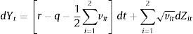


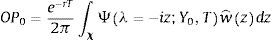
In this section I follow the methodology of Lewis (2000) and da Fonseca et al. (2007) to calculate option prices efficiently in terms of the generalized Fourier transform associated with the payoff function and with the asset return. In this sense, let us consider a generic payoff on the terminal value of the underlying asset, at time t=T, under the risk-neutral probability measure w(YT). From the Fundamental Theorem of Asset Pricing we have that the time t=0 price of this option, denoted OP0, is given by:
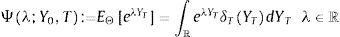
where δTYT is the risk-neutral density function of YT. The Laplace transform of the asset return is defined as: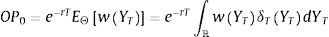
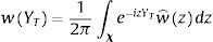
On the other hand, the Fourier transform corresponding to w(YT) is given by:
withwhere χ ⊂ ℂ is the admissible integration domain in the complex plain corresponding to the generalized Fourier transform associated with the payoff function wˆz and where i2=−1. Substituting previous expression in Eq. (3) yields:where we have used the Fubini theorem. From the previous equation, to obtain a semi-closed-form solution for the option price we have to calculate the Laplace transform of the asset return, as well as the Fourier transform associated with the payoff function.2.1.1The Laplace transform of the asset return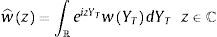
Marabel Romo (2013) shows that, under the risk-neutral measure Θ, the Laplace transform associated with the two-factor specification Ψ(λ;Y0,T) is given by:
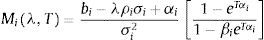
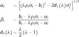
where Miλ,T for i=1, 2, is given by:with: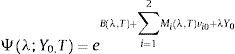
On the other hand, Bλ,T can be expressed as:
2.1.2The pricing formula for credit spreads and default probabilities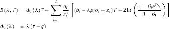
Let St denote the time t equity price corresponding to the firm. It is well known that, within Merton (1974) framework, it is possible to express the time t=0 equity price as a European call option on the firm's asset with maturity t=T equal to the expiration of the zero coupon bond with promised payment B, where this payment coincides with the option strike. From the put-call parity, it is possible to express the time t=0 debt value corresponding the firm, D0, as:
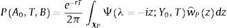
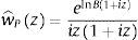
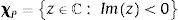
Hence, the debt value can be expressed as the difference between a zero coupon bond and a European put option on the firm's assets with strike equal to the debt payment at maturity P(A0, T, B). In this case, we can use the generic payoff Eq. (4) to express the time t=0 price of a European put with strike B and maturity t=T as follows:where χP ⊂ ℂ is the admissible integration domain in the complex plain corresponding to the generalized Fourier transform associated with the payoff functionUnder the assumption that Imz<0, where Imc denotes the imaginary part of c∈ℂ, the Fourier transform is given by:with the corresponding integrability domain:Therefore, we can combine Eqs. (5), (6) and (7) to obtain a semi-closed form solution for the price of a European put on the firm's assets. Note that the integral of Eq. (6) is an integral along a straight line in the complex plane. This line can lie anywhere in the region Imz<0. Since we know explicitly the marginal Laplace transform corresponding to the firms’ assets, it is also possible to obtain the price of European options using the fast Fourier transform method proposed by Carr and Madan (1999).

Taking into account the previous expressions, it is possible to express the time t=0 debt value:
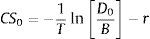
Therefore, the time t=0 credit spread, CS0, is given by:where D0 is given by Eq. (8).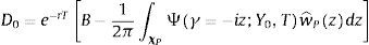
Within this framework, it is assumed that the firm defaults, at maturity t=T, if the firm's asset value AT is not enough to pay back the face value of the debt B to bondholders. As a consequence, the probability, at time t=0, of the firm defaulting at T, Pd0T, is given by:
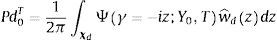
where 1. is the Heaviside step function or unit step function. In this case, we can express the default probability associated with the firm as follows:where χd ⊂ ℂ is the admissible integration domain in the complex plain corresponding to the generalized Fourier transform associated with the payoff function wˆdz, where the payoff function is:and, under the assumption that the assumption that Imz<0, the Fourier transform associated with the previous payoff function is given by:with the corresponding integrability domain:Hence, we can combine Eqs. (10), (11) and (12) to obtain a semi-closed-form solution corresponding to the default probability.3Numerical illustration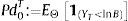

This section offers a numerical analysis of the ability of the two-factor specification to generate term structures corresponding to credit spreads consistent with empirical evidence. It also provides a study of the credit spread sensitivities with respect to the model parameters.
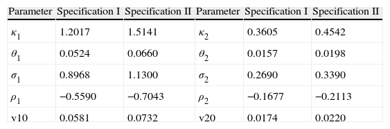
3.1The term structure of credit spreadsTo analyze the flexibility of the two-factor stochastic volatility specification to generate different patterns corresponding to the credit spread term structure, I consider the two parametric specifications of Table 1. Regarding the asset payout ratio q, the risk-free rate r, the initial firm's asset value A0 and the debt face value B, I take these parameters from Zhang et al. (2009). In this sense, I consider r=0.05, q=0.02 and A0=1. With regard to the debt face value associated with the parametric specification I of Table 1, I consider the debt face value corresponding to rating category A in the study of Zhang et al. (2009), whereas for the parametric specification II, I consider the debt face value corresponding to rating category BBB of Zhang et al. (2009). Hence, I set B=0.43 for specification I and B=0.48 for specification II.
Parameters specifications in the two-factor stochastic volatility model for firm's assets returns.
| Parameter | Specification I | Specification II | Parameter | Specification I | Specification II |
| κ1 | 1.2017 | 1.5141 | κ2 | 0.3605 | 0.4542 |
| θ1 | 0.0524 | 0.0660 | θ2 | 0.0157 | 0.0198 |
| σ1 | 0.8968 | 1.1300 | σ2 | 0.2690 | 0.3390 |
| ρ1 | −0.5590 | −0.7043 | ρ2 | −0.1677 | −0.2113 |
| v10 | 0.0581 | 0.0732 | v20 | 0.0174 | 0.0220 |
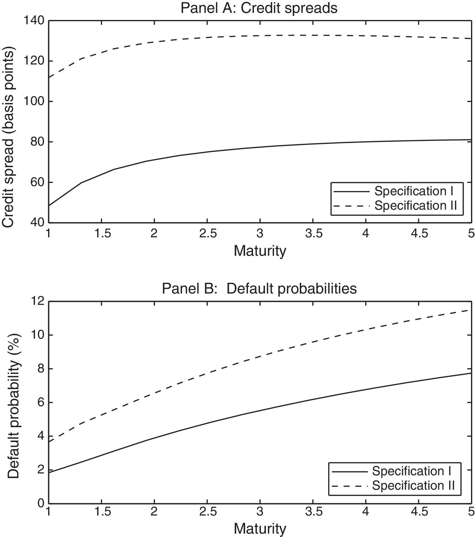
Panel A of Fig. 1 shows the generated credit spreads corresponding to each rating category for different maturities (expressed in years), whereas panel B displays the corresponding default probabilities. The credit spreads are calculated1 using the analytical expression of Eq. (9), while the default probabilities are calculated using Eq. (10).

Credit spreads term structure and default probabilities generated under the parametric specifications of Table 1. The figure has been generated using the following parameter values: r=0.05, q=0.02, A0=1 and finally, B=0.43 for specification I and B=0.48 under specification II.
The credit spread term structure generated by the two-factor model for specification I is of the same order of magnitude and it has a similar shape to the average credit spread term structure displayed by Zhang et al. (2009) in their sample of firms associated with the A rating category. Similarly, the term structure of credit spreads generated by the two-factor model associated with specification II, displayed in Fig. 1, is similar to the credit spread term structure corresponding to firms of credit rating BBB in the sample of companies considered by Zhang et al. (2009). Note that the difference between the default probabilities associated with both parametric specifications is increasing with the maturity. This effect is also consistent with the evidence presented by Zhang et al. (2009) using historical data on default probabilities. The examples of Fig. 1 show that the two-factor stochastic model is able to generate patterns corresponding to the credit spread term structure, as well as default probabilities consistent with empirical evidence. The advantage of this model with respect to single-factor specifications, such as the one used by Zhang et al. (2009), is that a two-factor model provides more flexibility to capture the volatility term structure since one of the factors determines the correlation between short-term firms’ assets returns and variance, whereas the other factor determines the correlation between long-term returns and variance. Hence, the two-factor specification is able to generate more flexible credit spread term structures to match the observed term structures associated with credit spreads.
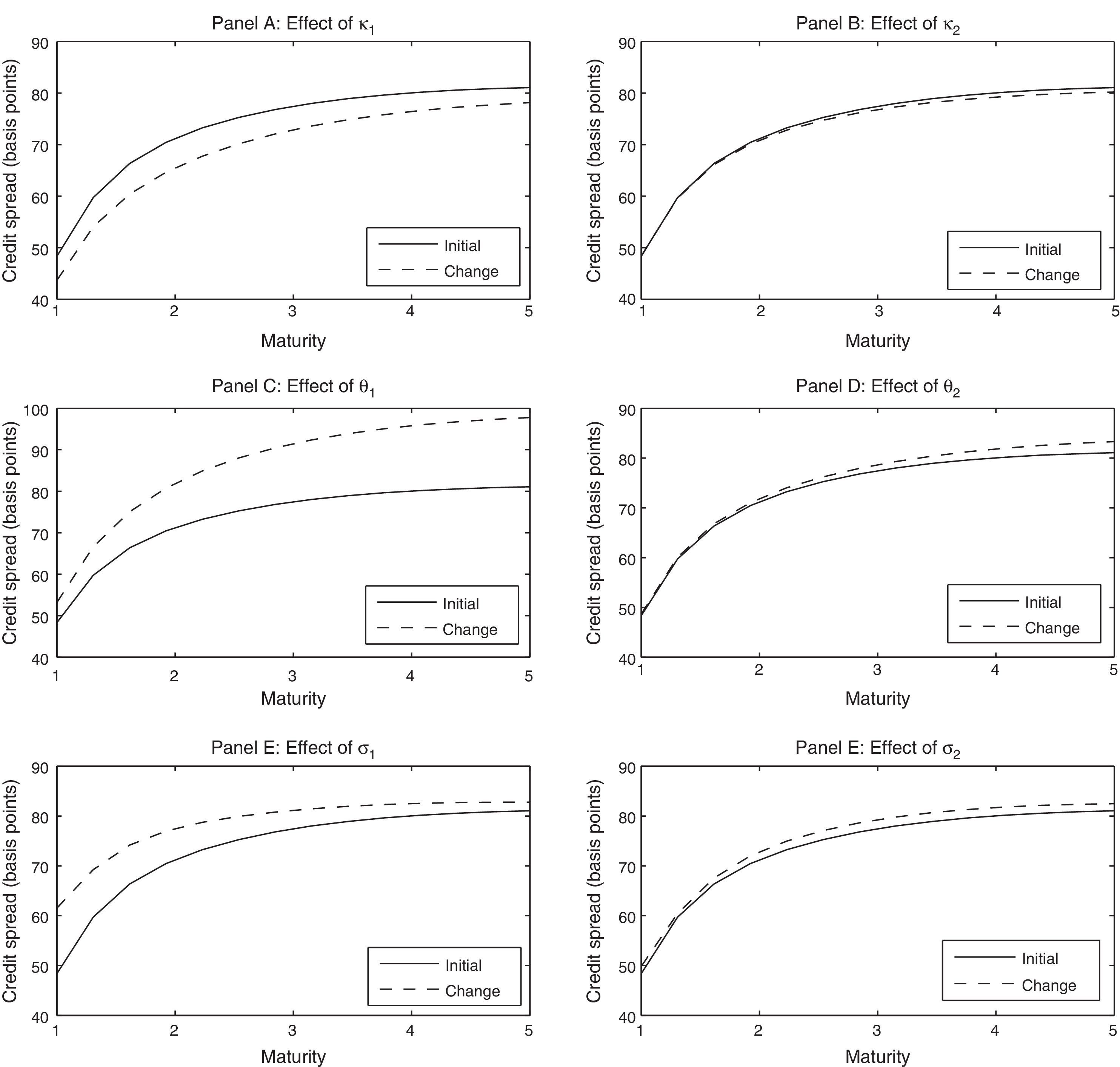
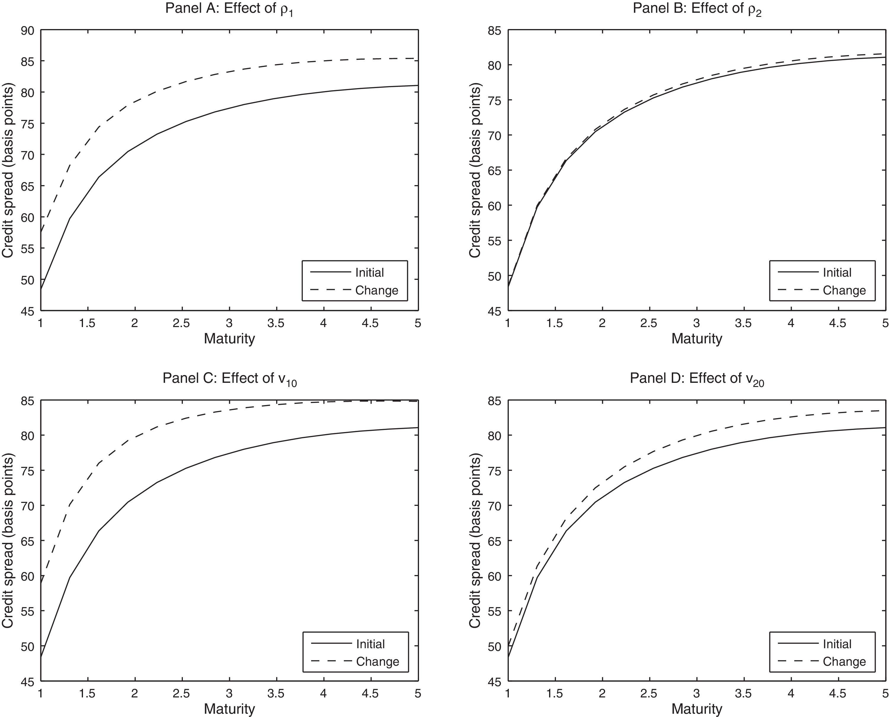
3.2Sensitivity analysisAs said previously, the two-factor stochastic volatility model provides more flexibility than single-factor specifications to model the volatility term structure and, hence, the credit spread term structure. This section considers the effects of the model parameters on the credit spread term structure associated with specification I of Table 1. In this sense, Fig. 2 provides the credit spread sensitivity with respect to the mean reversion parameters κ1 and κ2, the long-term variance factors θ1 and θ2, and, finally, the volatility of variance for each factor σ1 and σ2. On the other hand, Fig. 3 displays the sensitivities associated with the correlation coefficients ρ1 and ρ2, as well as the initial levels corresponding to each variance factor v10 and v20. The line initial shows the credit spread term structure associated with parametric specification I of Table 1, whereas the line change represents the credit spread term structure obtained when we multiply the corresponding parameter by the factor 1.25.

Sensitivity of credit spreads generated by specification I of Table 1 together with r=0.05, q=0.02, A0=1 and B=0.43.

Sensitivity of credit spreads generated by specification I of Table 1 together with r=0.05, q=0.02, A0=1 and B=0.43.
We can see from Fig. 2 that an increase in the mean reversion parameters reduces credit spreads. But in the case of κ1 the decrease of credit spreads is almost parallel for all maturities, whereas the change of κ2 only affects long-term spreads. Regarding the mean reversion parameters, both θ1 and θ2 increase the credit spread, especially in the long-term, but the effect of θ1 is more pronounced. With regard to the volatilities of the variance factors, σ1 increases above all the short-term credit spreads, while σ2 has impact especially in the long-term spreads. Higher correlation coefficients (in absolute value) and higher initial volatility levels for the variance factors imply higher credit spreads. But, as in the case of the mean reversion levels, the effect of the parameters associated with factor 1 on the term structure of credit spreads is almost parallel, whereas the second factor affects especially the long-term.
These numerical examples reveal how the introduction of two volatility factors can generate a wide range of combinations associated with short-term and long-term patters corresponding to credit spreads. In this sense, multifactor stochastic volatility specifications provide more flexibility than single-factor models to capture a wide range of shapes associated with the term structure of credit spreads.
4ConclusionThe empirical tests of traditional structural models of credit risk tend to indicate that such models have been unsuccessful in the modeling of credit spreads. To address these negative findings some authors, such as Zhang et al. (2009), introduce a single-factor stochastic volatility specification within the Merton (1974) framework. They show that their model improves the match between predicted and observed credit spreads, especially for investment-grade companies.
In the yield curve literature the use of multifactor models of the short rate is widespread. In fact, it is widely accepted in the literature that one-factor is not sufficient to capture the time variation and cross-sectional variation in the term structure. In this sense, it is perhaps somewhat surprising that multifactor models have not yet become more popular in the credit default literature. To fill this gap, this article introduces a two-factor stochastic volatility specification within the structural Merton (1974) model. The advantage is that a two-factor model provides more flexibility to model the volatility term structure. In this sense, one of the factors determines the correlation between short-term firms’ assets returns and variance, whereas the other factor determines the correlation between long-term returns and variance. The numerical tests reveal how the introduction of two volatility factors can generate a wide range of combinations associated with short-term and long-term patters corresponding to credit spreads. In this sense, multifactor stochastic volatility specifications provide more flexibility than single-factor models to capture a wide range of shapes associated with the term structure of credit spreads consistent with the empirical evidence. Future work will be devoted to the calibration of this model to market credit spreads.
The content of this paper represents the author's personal opinion and does not reflect the views of BBVA.
I have performed several numerical simulation tests to verify that the option prices obtained from the semi-closed-form solution presented in this article match perfectly with those produced with Monte Carlo simulations. Regarding the Monte Carlo specification, I consider daily time steps and 50,000 trials and I implement the quadratic exponential scheme as described in Andersen (2008). Moreover, I have implemented the pricing equations through the fast Fourier transform proposed by Carr and Madan (1999) obtaining the same results.

