Logistic regression models

Abstract

In the health sciences it is quite common to carry out studies designed to determine the influence of one or more variables upon a given response variable. When this response variable is numerical, simple or multiple regression techniques are used, depending on the case. If the response variable is a qualitative variable (dichotomic or polychotomic), as for example the presence or absence of a disease, linear regression methodology is not applicable, and simple or multinomial logistic regression is used, as applicable.

Introduction

In the early 1960s, Cornfield et al.¹ were the first to use logistic regression (LR). In 1967, Walter and Duncan² used this methodology to estimate the probability of occurrence of a process as a function of other variables. The use of LR increased during the 1980s, and at present it constitutes one of the most widely used methods in research in the health sciences, and specifically in epidemiology.

One of the aims in epidemiology is to study those factors which at a given moment affect the existence of a health problem, and to control the dimension of the latter, as well as to construct models with predictive capacity that can assess the mentioned health problem.

The objective of this procedure is to establish the best model for explaining a qualitative dichotomic variable Y [0,1], called a response or dependent variable, that will serve to explain whether an individual has a health problem or not, based on another series of variables called covariables, predictor variables or simply independent variables X₁, X₂, X₃, …, X_m indicating the characteristics of the subject, and which may be both discrete and continuous. When the response variable (Y) is of the dichotomic type, we refer to logistic regression, and when the dependent variable (Y) is qualitative with more than two categories (polychotomic), we refer to multinomial logistic regression.

The logistic regression model is very appropriate for addressing issues of this kind, provided a sufficiently numerous and well-distributed sample is available. In addition, in designing the study, and following an adequate literature search and with good knowledge of the subject, all the important variables for explaining the response variable must be taken into account.

In addition to avoiding the limitations of linear regression when the result variable is dichotomic, this technique makes it possible to interpret the parameters in an easy manner in terms of odds ratios (ORs).

The present article describes binary and multinomial logistic regression, its calculation, and checking of the assumptions for application, accompanied by an illustrating example with the shareware R program³.

Prior definitions

Before starting with the logistic regression model, a reminder will be provided of a series of concepts, which later on will contribute to understanding the article better.

Risk or probability

The number of cases in which the event occurs, divided by the total number of cases or risk of occurrence of the event.

Example: 20 out of every 200 newborn infants have asthma. The risk of asthma is therefore 20/200 = 10%.

Odds

The number of cases in which the event occurs, divided by the number of cases in which the event does not occur.

Continuing with the previous example: odds of asthma = 20/180.

The risk of having offspring with asthma is seen to increase in smoking women, with a frequency of 10 cases out of every 40 smoking women. In this example the risk = 10/40 and odds of asthmatic newborn infant (NB) = 10/30.

For measuring the intensity of the relationship between a given type of exposure (smoking) and a certain effect (asthmatic NB), we use “measures of strength of association”. These measures of association never measure causality, vary according to the design of the study, and are represented by the relative risk and odds ratio.

Relative risk (RR)

Ratio between the risk of asthmatic NBs of smoking mothers and asthmatic NBs of non-smoking mothers.

Example: RR = (10/40)/(20/200) = 2.5.

Odds ratio

Ratio between the odds of asthmatic NBs exposed to smoking mothers and the odds of asthmatic NBs not exposed to smoking mothers.

Example: OR = (10/30)/(20/180) = 3.

The RR is intuitive and easier to interpret than the OR, although the latter is easier to calculate and can be made in any design, since RR cannot be used in case-control or retrospective studies.

The usual approach is to determine whether the existing conditions are suitable for allowing OR to be a good estimator of RR, and in this case we calculate OR and interpret it as RR.

In order for OR to be a good estimator of RR, the following must apply:

• a)

  The frequency of disease is low (<10%).⁴

• b)

  The controls are representative of the population from which the cases are drawn.

• c)

  The cases offer good representation of the population of cases. To this effect it is always preferable for the cases to be incident cases, not prevalent cases, i.e., new cases rather than cases already observed at the start of the study period.

Let us examine the interpretation of these two measures:

• RR = 3 indicates that smoking women are three times more likely to have asthmatic offspring than non-smoking women.

• RR = 1 indicates that there is no association between the effect (smoking mother) and the cause (asthmatic NB).

• RR > 1 indicates that there is a positive association, i.e., the presence of the risk factor is associated to a greater frequency of the event.

• RR < 1 indicates that there is a negative association, i.e., there is no risk factor, but rather a protective factor.

Both RR and OR have no dimensions and take values between zero and infinity. Thus:

• OR = 1 is interpreted as indicating that there is no such risk factor, since the odds for the exposed are the same as those for the non-exposed.

• OR > 1 is interpreted as indicating that there is a risk factor, since the odds of the event occurring in response to exposure to the factor are greater than in the case of non-exposure.

• OR < 1 is interpreted as indicating that the odds of the event occurring in those exposed to treatment are lower than in the case of those not exposed to treatment, and thus we are in the presence of a protective factor.

• OR has no dimensions and takes values between zero and infinity.

Binary logistic regression

The logistic regression model

Logistic regression models are statistical models in which an evaluation is made of the relationship between:

• -

  A dependent qualitative, dichotomic variable (binary or binomial logistic regression) or variable with more than two values (multinomial logistic regression).

• -

  One or more independent explanatory variables, or covariables, whether qualitative or quantitative.

In this section we describe the situation in which we start with a response variable (dependent variable) with two possible values (become ill or not become ill), and wish to examine the effect upon it of other variables (predictors or independent variables).

Definition of the best model depends on the type and objective of the study. The model usually has two types of objective: predictive or explanatory.

In a model with predictive objectives we aim to establish a parsimonious model, i.e., a model involving the least number of variables that best explain the dependent variable.

In the case of a model with explanatory objectives, we aim to study the causal relationship between a “cause” variable and an “effect” variable, with due control of the possible confounding variables (defined in Section ‘Interaction and confounding factors’) or effect modifying variables (interaction) in this causal relationship.

It is important to take this into account, since it leads to completely different modelling strategies. Thus, in the case of a predictive model, the best option is a model offering more reliable predictions, while in the case of a model aiming to estimate the relationship between two variables, the best option is considered to be a model offering a more precise estimation of the coefficient of the variable of interest.

In explanatory models with variables presenting statistically significant coefficients but whose inclusion in the equation of the model does not modify the value of the coefficient of the variable of interest, these will be excluded from the equation, since no confounding factor is involved in the causal relationship between the “cause” and the “effect” variables, and thus the relationship between these two variables is not modified if the third variable is taken into account.

In predictive models, if we have a variable with statistically significant coefficients, it is included in the equation, since in this case we are seeking more reliable predictions.

A logistic regression model is very useful in the following circumstances:

• -

  Given a set of values of the independent variables, we wish to estimate the probability that the event of interest will occur (e.g., falling ill).

• -

  Evaluation of the influence each independent variable has upon the response, in the form of OR (since this is the value resulting from the equation).

Construction of the model:

We start from the univariate case, i.e.:

• -

  Y: dichotomic dependent variable, with response 0 when the event does not occur (absence of event) and response 1 when the event is present (event).

• -

  X₁: independent variable, which may be of any nature, qualitative or quantitative.

We wish to relate the true proportion p of individuals presenting a certain characteristic (e.g., being ill) to the value of a certain explanatory variable X₁ as possible risk factor. If linear regression is performed, and in order to use the data to estimate the coefficients β₀β₁ of the equation:

The above leads to absurd results, since p takes values between 0 and 1, while in the regression model we assume that p follows a normal distribution and therefore should be between −∞ and +∞. In order to avoid this problem, it is common to define a binding function f(p) between −∞ and +∞, and then see whether we can assume the classical lineal model.⁵ In this way a normal distribution for the dependent variable f(p) is obtained, transforming the above equation into the expression:

where “e” are the residuals, i.e., the variability not explained in the model, as defined in the linear regression article.⁵

In the statistical setting it is common to use logit transformation: f(p) = ln{p/(1 − p)}. With this transformation, the simple logistic model is:

Or, equivalently:

For the multivariate case, the above expression is generalised to the case in which there are k independent variables or risk factors (X₁, X₂,…X_k), based on the expression:

Or in terms of probability:

The exponentials of the coefficients β_i associated to the independent variables are interpreted as the OR of suffering the disease in question (or of occurrence of the event) for each increase in the independent variable, adjusting for the rest of independent variables.

The truly important aspect of the logistic regression model is that we can jointly analyse various factors or variables, with a view to examining how they can affect occurrence or non-occurrence of the study event.

Coding and interpretation of the coefficients of the model

Coefficients of the logistic model as risk quantifiers

It is advisable to adhere to the following recommendations when coding the variables of a logistic regression model, since it facilitates interpretation of the results:

• -

  Dependent variable: we code as 1 the occurrence of the event of interest, and as 0 the absence of the event. Example: 1: disease yes, 0: disease no.

• -

  Independent variables: these may be of different types:

  • -

    Numerical variable: in order to introduce the variable in the model, it must satisfy the linearity hypothesis,⁶ i.e., for each unit increase in the numerical variable, the OR (exp B_j) increases by a constant multiplicative value. In this case we can use the variable as it is in the model.If the linearity hypothesis is not met, we can transform the numerical variable, categorising it.When the variable is continuous, the associated OR is interpreted as the increase in risk per unit increase in the analysed covariable, i.e., if the risk factor were age, the result variable would be having or not having the disease, and if the OR were 1.87, then this value would be interpreted as indicating that for each additional year of age of the subject, the risk of suffering the disease increases by 1.87. In other words, the probability of suffering the disease increases 87% for each additional year of age, adjusting for the rest of variables of the model in the multivariate case.This is seen to be a model in which the increase or decrease in risk on changing from one factor value to another is proportional to the change, i.e., to the difference between the two values, but not to the starting point.

  • -

    Dichotomic variable: we code as 1 the case believed to favour occurrence of the event, while the opposite case is coded as 0, i.e., we code as 1 those individuals exposed to a supposed risk factor, and as 0 those individuals not exposed to the mentioned factor.Thus, if we code smoking mothers as 1 and non-smoking mothers as 0, and the event of interest is taken to be an asthmatic child (coded as 1) versus a non-asthmatic child (coded as 0), and we obtain OR = 2.23, then it can be concluded that smoking mothers are at a 2.23-fold greater risk of having an asthmatic child than non-smoking mothers. Alternatively, this can be interpreted as indicating that the risk of having a child with asthma in the case of a smoking mother is a little over twice as great as in the case of a non-smoking mother, in all cases adjusting for the rest of covariables of the model.

  • -

    Categorical variable: this type of variable is divided into different dichotomic variables representing the different categories. These variables are known as indicator, internal variables, design variables or “dummy” variables. Most statistical software applications generate these variables internally on including a factorial type variable in the model (i.e., with more than two categories).In this type of codification we usually select a reference category, and the coefficient of the regression equation for each “dummy” variable (always transformed with the exponential function) corresponds to the OR of that category with respect to the reference level. Thus, we quantify the change in the risk of suffering the event of each of the categories with respect to the reference category. Accordingly, and continuing with the previous example, if the variable of smoking is taken to have three categories: never smoked, ex-smoker, and active smoker, and we take as reference the category “never smoked”, then we will obtain the risk of having an asthmatic child among ex-smoking mothers versus the mothers who have never smoked. In turn, we will obtain the risk of having an asthmatic child among the mothers who are active smokers versus the mothers who have never smoked.

When coefficient β of the variable is positive, we obtain OR > 1, and it therefore corresponds to a risk factor. If the value β is negative, OR will be <1, and the variable therefore corresponds to a protective factor.

In other words, exp(β) is a measure that quantifies how much more risk of suffering the event is present in the individual with the risk factor versus the individual without the risk factor.

Interaction and confounding factors

A confounding factor is a variable that satisfies three conditions:

• 1)

  It is a risk factor for the effect under study.

• 2)

  It is associated with the exposure under study.

• 3)

  It is not an intermediate link in the a priori postulated causal chain between exposure and effect.

The presence of risk factors generates bias in evaluating the relationship between independent and dependent variables.

Interaction exists when the magnitude of the association between a given exposure and an effect “changes” according to the magnitude of a third variable, referred to as an “effect modifier”. If detected, it must be included in the model independently with respect to the effect modifier variable (through the cross-product of both variables).

Logistic regression models allow the introduction of adjusting variables for confounding factors and interaction, and can contain higher grade terms such as for example (age²), transformations such as for example (ln age), and also interactions such as for example (age × smoking).

Interpretation of the coefficients associated to the interaction is somewhat more complicated than in the previous cases. In the example of mothers with asthmatic children, if we have an OR associated to the interaction covariable (age_mother × smoking) of 1.05, it could be interpreted that for smoking mothers, the risk of having an asthmatic child increases 5% for each year of increase in the age of delivery of the mother.

In order to evaluate the confounding effect, we simply construct two models: one including the possible confounding factor and the other without the confounding factor – observing the difference between the OR in one model and the other.

In order to determine a possible modification of effect or interaction of one variable with respect to another, the simplest approach is to include a new variable represented by the product of the two implicated variables in the model. This yields a new coefficient associated to this new variable, and if the partial contrast of this coefficient is statistically significant, we will consider that interaction indeed exists. It must be taken into account that in addition to the interaction variable, we also introduce those two variables in the model separately.

Validation, hypothesis and selection of the model

On comparing logistic regression with linear regression, the former offers the advantage of not having to satisfy assumptions such as the existence of a linear relationship between the response and the predictor variables, normality and homoscedasticity of the residuals. The essential assumptions of logistic regression are independence between the successive observations and the existence of a linear relationship between logit(x) and the predictors X₁, X₂, …, X_k.

One of the necessary considerations before applying the logistic regression model is to determine whether the relationship between the independent variable and the probability of the event changes its sense or direction, or not. An example of this is when we have a situation where for small values of the independent variable an increase in this variable also increases the dependent variable, while from a certain value of the independent variable an increase in the latter leads to a decrease in the dependent variable. If this happens we cannot apply the model, although in the absence of this change in sense or direction the logistic model would be adequate.

We must also consider possible situations of colinearity, which occurs when the model contains strongly correlated independent variables – leading to a meaningless model, and thus to non-interpretable coefficient values.

Another point to be taken into account when constructing a logistic regression model is the size of the sample. It will be necessary to have at least 10 × (k + 1) cases in order to estimate a model with k independent variables.⁷ We must take into consideration that in the case of a qualitative variable with j categories, we introduce j − 1 “dummy” variables in the model, which will be regarded as j − 1 variables when considering the number of cases required for construction of the model.

Construction of the logistic model is carried out using maximum likelihood methods. The models based on maximum likelihood methods are those, which maximise the probability of obtaining the observed data, derived from the adjusted model. These methods involve the construction of the likelihood function (which, depending on the type of regression used, will be more or less complex, and is strongly tied to the distribution of the observed results) and maximisation of its result. This is equivalent to calculating the coefficients of the model in a way that best explains the data obtained. Due to the complexity of the maximisation problem to be resolved, we need to use iterative methods to find a solution. Based on the likelihood function, we can calculate the deviation (or deviance) as −2 × logarithm of the likelihood function. In this way maximisation of the likelihood function becomes a problem of minimisation of the deviation (simplifying the problem of optimisation).

In constructing the model, we must first consider the parsimonious model. To this effect we determine all the independent variables that can form part of the model (considering also the possible interactions). For discriminating the variables to introduce in the model, it is advisable to previously and separately study the relationship of each factor with the dependent variable. The model should include the variables found to be statistically significant in the bivariate analysis, the confounders, and the clinically relevant parameters.

There are several methods for the inclusion of variables in the model,⁸ although the following three are the most common: (a) starting with a single independent variable, and then adding new variables according to a pre-established criterion (forward procedure); (b) starting with the maximum model, followed by the elimination of variables according to a pre-established criterion (backwards procedure); and (c) the so-called “stepwise” procedure, which combines the above two methods, and where in each step we can add or eliminate another variable that was already present in the equation.

The logarithm of the likelihood ratio of the models is the criterion selected in each step of the construction of the model in order to determine whether a new model is to be chosen versus the current model. The smaller the likelihood value, the better the model, although there is no adequate minimum value. The likelihood function is a measure of the compatibility of the data with the model; thus, if on adding a variable to the model the likelihood does not improve to a statistically significant degree, then this variable should not be included in the equation.

Goodness of fit

In a logistic regression model, having estimated the latter by means of the maximum likelihood method, the global fit is described with statistics derived from the likelihood of the model.

There are different statistics that describe the global fit of the model to the data. One of them is the −2log likelihood = −2LL. If the fit of the model were perfect, then −2LL = 0. In other words, this value can be regarded as a descriptor of the goodness of fit of this model, and the closer it is to zero, the better the fit of the model.

There are two indexes that represent the proportion of uncertainty of the data explained by the adjusted model. Through analogy with the determination coefficient in the linear regression, they are represented by R² corresponding to the R² of Cox and Snell⁹ and the R² of Nagelkerke.¹⁰

The value of the R² of Cox and Snell⁹ has the inconvenience of not reaching the value 1 (100%) when the model reproduces the data exactly.

For this reason, Nagelkerke proposed the corrected R² of Nagelkerke,¹⁰ which yields a value of 1 if the model explains the 100% of the uncertainty of the data:

Another measure that describes the global fit of the model is the chi-squared goodness of fit test. This is a chi-squared goodness of fit statistic that compares the observed values Y_i with the values p(x_i) predicted by the model.

The above indicators of goodness of fit have been presented from a purely descriptive perspective in relation to fitting of the model.

Since the model has been estimated by the maximum likelihood method, its global significance, i.e., the significance of the set of included predictor variables, is assessed with the so-called “likelihood ratio test”.

The likelihood ratio test for studying the significance of the model involves comparing the goodness of fit of the saturated model (including all the variables) with the null model (adjusted by a constant) through the deviations ratio (deviance = −2log(likelihood)). We thus construct a statistic that follows a chi-squared distribution with (number of variables of the saturated model − 1) degrees of freedom (df).¹¹

An analogous procedure could be considered for testing the significance of the coefficient associated to a covariable by simply comparing the complete model with the model excluding the covariable of interest. Wald demonstrated that the sample distributions of the maximum likelihood estimations of the parameters β are distributed according to normal laws when the samples are large. Thus, the significance of the parameters can be studied with the ratio z = B/SE(B), which follows a standardised normal distribution, or with the square of this ratio, which is known as the Wald statistic,¹² and follows a chi-squared law:

The likelihood ratio test is more powerful than the Wald test. Different studies^13,14 have demonstrated the lack of power of this test when the value of the parameter β moves away from zero, and recommend that a likelihood ratio test (−2ln LR) should be used instead.

The calibration of the model is an aspect of the fit that assesses concordance between the probabilities observed in the sample (p_i) and those predicted by the model (Π_i). A contrast has been developed which evaluates the general calibration of the model based on the expected frequencies and the frequencies predicted by the model (Hosmer–Lemeshow).¹⁵

However, in some statistical programs, such as the program R, use is made of the modified le Cessie–van Houwelingen statistic,^16,17 which is a modification of the Hosmer–Lemeshow statistic.

Multinomial logistic regression

The logit multinomial regression models are the extension of the logistic models in the case where we study a categorical dependent variable with more than two possible responses.^6,18

If we wish to adjust, predict or estimate the possible values of a polychotomic response variable Y (with more than two possible discrete values Y₁, Y₂, …, Y_m) from a set of predictor variables (one or more covariables X₁, …, X_n), we use models of this kind.¹⁹

In these models there are no prior hypotheses on the distribution of the dependent variable, and they therefore are ideal when we have a categorical variable with more than two possible responses.

The rationale followed for estimation of the model is equivalent to estimating a system of m − 1 logistic equations comparing in each equation each of the possible values of the response variable with the reference value pre-established by the investigator.

For example, suppose we wish to relate the variable weight at birth of a newborn infant, categorised as <2000 g, 2000–3500 g and >3500 g, to the independent variable smoking mother (yes/no). In this case we fit a system of two logistic models. If we establish as reference value the category >3500 g, then one of the logistic models evaluates the risk of birth weight <2000 g versus the category >3500 g, controlling for the variable smoking mother. In the same way we construct the second regression equation, comparing the risk of weighing between 2000 and 3500 g, versus the risk of weighing more than 3500 g, in the case of a smoking mother versus a non-smoking mother. On resolving the system of logistic equations we cover the entire set of possible values of NB weight.

where:

• p₁ refers to the proportion of NB that weigh <2000 g versus the reference group (NB weighing >3500 g).

• p₂ refers to the proportion of NB that weigh between 2000 and 3500 g, likewise compared with the same reference group.

• X refers to smoker or non-smoker status of the mother.

Example R

Univariate model

“In the same study population of the multinomial example we wish to determine the effect of having an asthmatic mother (asmother) upon possible asthma in the NB (whezev)”

In the presented example we have the following variables:

• Asmother (independent variable):

  • •

    1 Asthmatic mother (can be labelled as Yes)

  • •

    0 Non-asthmatic mother (can be labelled as No)

• Whezev (dependent variable):

  • •

    1 Asthmatic NB (can be labelled as Yes)

  • •

    0 Non-asthmatic NB (can be labelled as No)

In order to define the model we use the function glm, which defines a generalised lineal model²⁰:

GLM.1<-glm(whezev∼asmother,family=binomial(logit),data=Data)

The function glm adopts the following arguments:

Formula: we specify the functional form of the model we wish to adjust as Y ∼ X₁ + ··· + X_n.

Family: we specify the link function associated to the generalised lineal model or, in other words, we indicate the type of regression we wish to apply (in the case of logistic regression we select the binomial(logit) family).

Data: we enter the name of the data frame where the study variables are filed.

Note that we have filed the logistic model in the object GLM.1.

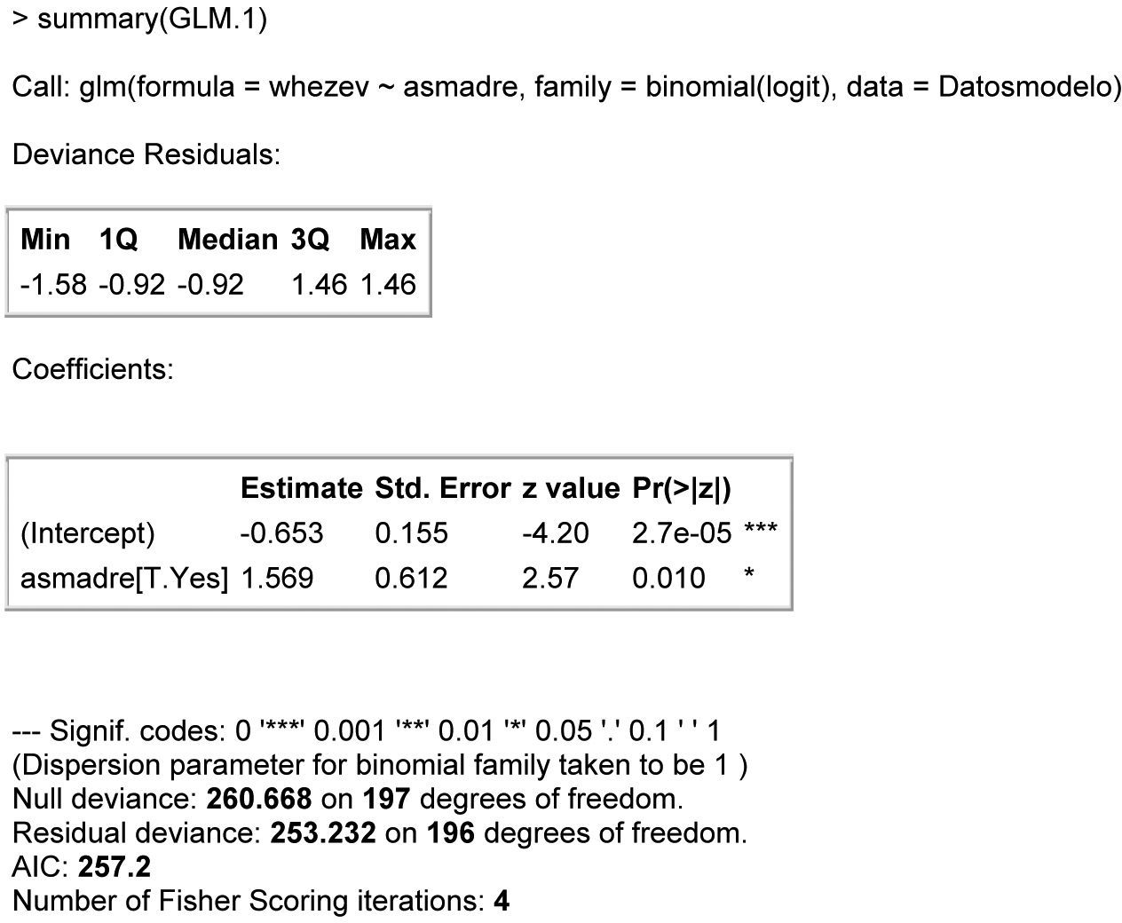
We can produce a summary of the model by resorting to the summary function. This summary can be seen in Fig. 1, showing:

• 1.

  The function used to calculate the model.

• 2.

  A descriptive summary of the residual standard deviation of the model (Deviance Residuals), where we see whether the errors of approximating the obtained values to those predicted by the model are around the value zero – indicating general goodness of fit of the model to the data obtained.

• 3.

  Estimated coefficients of the model (Estimate), standard error associated to the estimation of the coefficient (S.E.), value of the statistic associated to contrast of the null hypothesis of the associated coefficient (z-value) together with the associated p-value (Pr(>|z|)) and a code expressing the level of significance (α) for which the mentioned coefficient would be significantly different from zero.

• 4.

  The associated coefficient is significantly different from zero (and therefore represents a factor that influences the response variable) if the associated p-value is lower than the level of significance pre-established by the investigator and identified in the statistical summary by the number of asterisks.

• 5.

  Lastly, information is provided related to the general degree of fit of the model, where:

  • •

    Null deviance refers to the deviation residual associated to the current model with its degrees of freedom.

  • •

    Residual deviance refers to the deviation residual associated to the adjusted model with its degrees of freedom.

Figure 1.

Simple Logistic regression model with a categorical covariate.

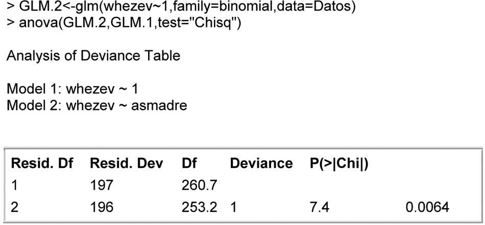
From these values we can calculate the general degree of fit of the model via the goodness of fit, based on the likelihood ratio of the model, Fig. 2. Note that in the table appearing at this output, significance is obtained for the contrast based on the likelihood ratio test – thus indicating that globally, the variable asthma mother contributes relevant information for predicting the dependent variable asthma NB.

Figure 2.

Goodness of fit test of the model GLM.1.

Lastly, we can make use of the logistic.display( ) function of the epicalc package,²¹ which adopts as argument a logistic model of the above form and returns a table with the most interesting information in clinical terms, summarised in Fig. 3.

Figure 3.

Summary of the logistic model GLM.1.

In this output we see:

The dependent variable used in the model with the comparison category versus the reference category used in the model (the R program always uses as reference category that with the least associated number value), along with the covariable used in the model indicating comparison value versus reference value, the odds ratio associated to the covariable together with the associated 95% confidence interval (95%CI), and the p-value of the contrast statistic associated to the null hypothesis of the preferable coefficient (P(Wald) and P(LR-test) when there are few cases per comparison category).

Interpretation of the model:

The model obtained at Fig. 3 can be expressed as:

logit(whezev) = coefficient (intercept) + coefficient(asmother) × asmotherwhere

• -

  coefficient(intercept) = −0.653;

• -

  coefficient(asmother) = 1.569;

• -

  whezev and asmother initially defined variables;

• -

  Logit(whezev) = log(p/1 − p), where p = probability that a NB of the sample is asthmatic.

In this way we can interpret the risk of asthma in a NB of an asthmatic mother as being exp(1.569) times that of the case of a non-asthmatic mother. In other words, the risk of asthma for a NB of an asthmatic mother is 4.8 times greater than in the case of a non-asthmatic mother.

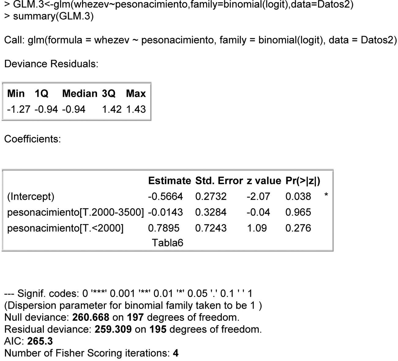
Polychotomic covariable (or discrete with more than two possible categories)

Weight at birth of the multinomial example is regarded as a factor associated with asthma in the newborn infant.

In this case we would have to include as many “dummy” variables as categories – 1 of the associated variable.

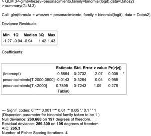
This is done automatically by the R program, and we only have to indicate the name of the variable where it is defined. The only point we have to take into account is that the polychotomic variable must be of the factorial type; see Fig. 4.

Figure 4.

Simple logistic regression model with a politomous covariate.

The information obtained in the case of a dependent polychotomic variable is the same as in the dichotomic case but including each of the “dummy” variables auto-calculated by the program.

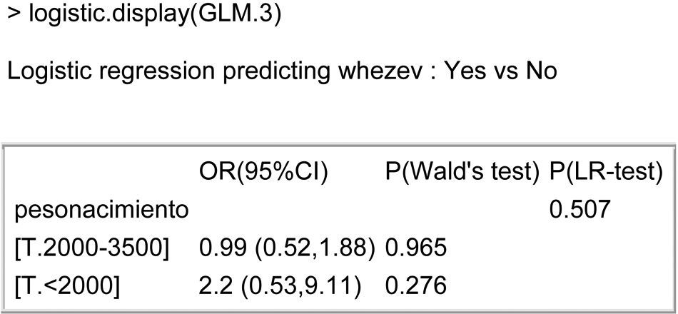
Using the logistic.display( ) function we can obtain a single table offering the information relating to each of the covariables of the model; see Fig. 5. Thus, the risk of asthma in a NB weighing <2000 g doubles when compared with a NB weighing >3500 g (even if the difference is not significant and we therefore cannot be sure of the correctness of the result).

Figure 5.

Summary of the model GLM.3.

Continuous covariable

Here we wish to relate a continuous or numerical variable to the dependent variable asthma in the infant. We consider in this case the forced expiratory volume in one second (fev1) as covariable of the model.

We first must check the linearity of the continuous variable, whereby proportional increments of the independent variable lead to proportional increments in the odds ratio. To this effect we can categorise the continuous variable into several categories and check that there is certain linearity in the coefficients associated to the model obtained on adjusting the dependent variable to the categorised variable.

The function cut( ) adopts the following arguments:

Data: continuous variable we wish to categorise into subgroups.

No. of categories (b): with this parameter we indicate the number of categories we wish to obtain.

The function returns a variable with different no. of categories of equal length from the variable data.

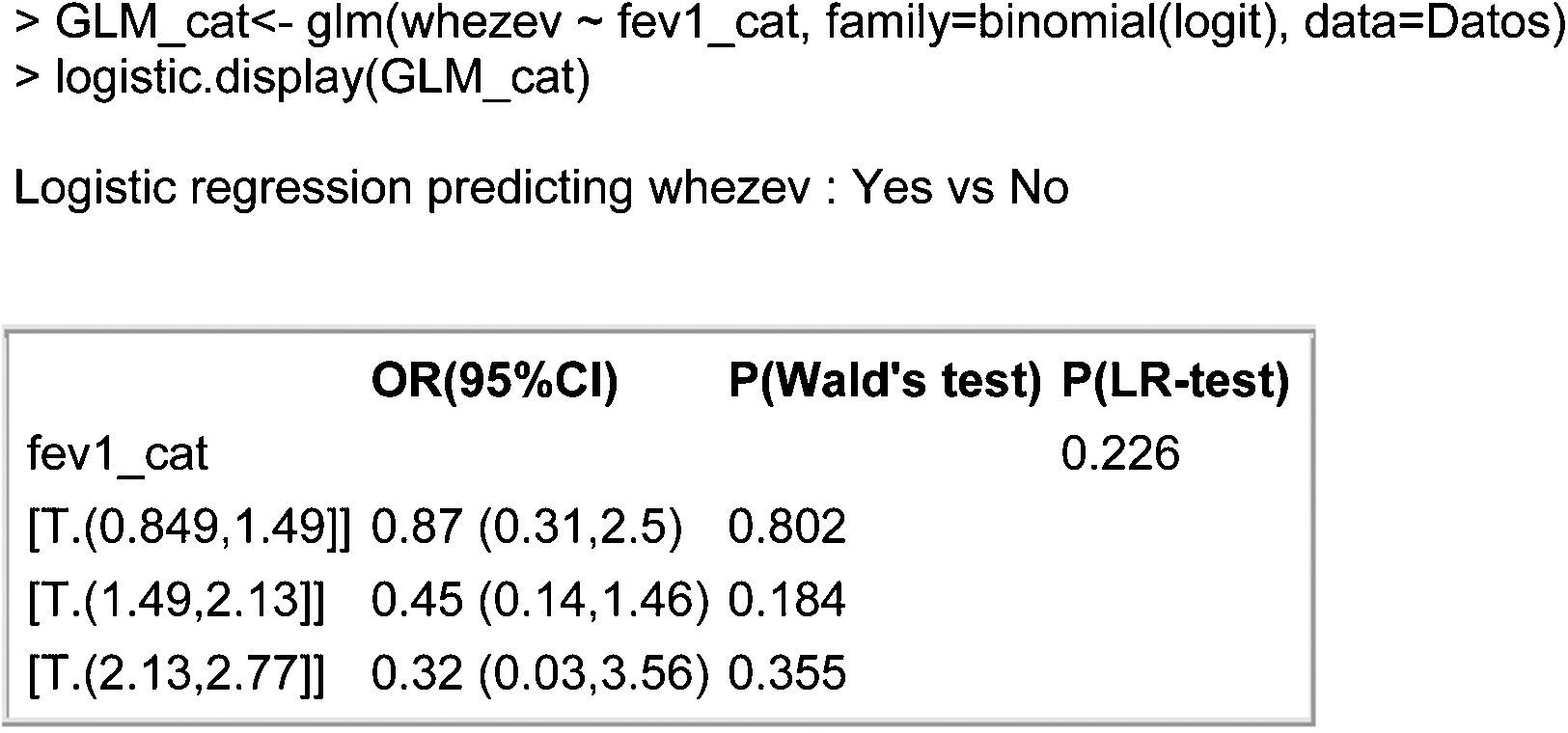
The model obtained can be seen in Fig. 6. The table shows that the OR associated to each of the categories decreases as the % exhaled volume increases. This result corroborates the linearity hypothesis of the continuous variable, as we therefore can include it as continuous variable in the model, as can be seen at Fig. 7. The output shown in the table indicates that the risk of suffering asthma decreases 0.44-fold for each one-unit increase in the spirometry result (or, in other words, a one-unit increase in the spirometry response increases the odds of not suffering asthma a little over 2-fold; 1/0.44 = 2.27).

Figure 6.

Model to check the linearity of the continuous covariable.

Figure 7.

Logistic regression model with a continuous covariable.

It should also be mentioned that although the categorised continuous variable does not contribute relevant information to the model (P-LR test = 0.226 > 0.05), the continuous variable does prove significant. This is because when grouping a continuous variable we always run the risk of losing information due to poor categorisation of the variables.

Multivariate model

Continuing with the above example, we perform a multivariate analysis for the result variable asthma in the NB.

To this effect we have selected an iterative forwards and backwards stepwise criterion for the selection of variables based on the criterion of minimisation of the AIC,⁵ starting from an intermediate model including the variables weightbirth, sex (sex of the NB) and smokermother. Posteriorly, we evaluate the rest of the study variables, and finally the resulting multivariate model is produced at Fig. 8. As can be seen in the table, the variables influencing the development of asthma in the NB are whether the mother smokes and whether the mother has asthma.

Figure 8.

Multivariate logistic regression model.

The results obtained show that:

• -

  The risk of suffering asthma in a NB with a smoking mother is 56% greater than in the case of a non-smoking mother, for equal asthmatic condition of the mother.

• -

  The risk of suffering asthma in a NB with an asthmatic mother is more than five times the risk in the case of a NB with a non-asthmatic mother, for equal smoker condition of the mother.

• -

  Lastly, if we wish to compare the risk of asthma in a NB with an asthmatic and smoking mother versus the case of a mother who neither smokes nor has asthma, we simply calculate 1.56 × 5.22 = 8.14. Thus, a smoking mother with asthma is eight times more likely to have an asthmatic child than a mother who neither smokes nor has asthma.

For validation of the model, we can again compare the calculated model with the null model, or alternatively as commented in the section on goodness of fit, we can calculate the Hosmer–Lemeshow statistic as modified by Cessie–van Houwelingen.

We load the foreign²² and Design²³ libraries needed for calculation of the statistic.

In order to calculate this statistic we must calculate the matrix of design and the response variable associated to the adjusted model.

Lastly, we use the function residuals.lrm to specify the type of contrast of goodness of fit we wish to obtain; see Fig. 9. The table shows that since the contrast does not prove significant (p-value = 0.587), there is no statistical evidence of an absence of fit of the data to the model.

Figure 9.

Goodness of fit test.

Multinomial model

Returning to the example commented in the theoretical development of the model, we define the model based on the multinom function:

This adjusts a multinomial model by means of the formula Dependent variable ∼ Covariables, of the set of data specified in the second argument data=B.D. The command trace refers to whether we wish to observe parameters of the iterative maximum likelihood method of the fit of the model (based on neural networks).

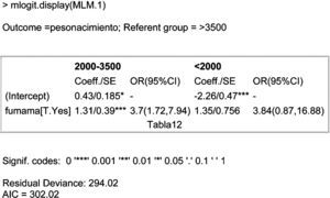
We select the mlogit.display function of the epicalc package for obtaining a representation of the model that is more interpretable at clinical level; see Fig. 10. A description is given below of the table that appears at the mentioned output:

Figure 10.

Multinomial logistic regression model.

Outcome and referent group (result variable and reference group)

We see that on comparing all with the reference group of greatest weight (>3500 g), what we are evaluating are factors that influence weight loss in the NB.

Row 1 (R1). – coefficient of interception (intercept, independent term or constant) of each of the adjusted models (comparing weights of 2000–3500 g versus >3500 g, and comparing weights of <2000 g versus >3500 g), standard error associated to each coefficient.

R2. – coefficient associated to the covariable entered in the model (smokermother[T.Yes] = compares smoking mother versus non-smoking mother), standard error, relative risk and confidence interval associated to the covariable smoking mother (smokermother).

The degree of statistical significance associated to each of the coefficients can be seen by means of the code of the number of asterisks in each of them.

Lastly, we have information relating to the general degree of fit of the model (Residual Deviance and AIC).

Thus, the first column (associated to the first comparison model) of the summary, given by the mlogit.display function, can be expressed as:

where OR(2000–3500 g/>3500 g) is the risk associated to weighing between 2000 and 3500 g, given that the NB weighs more than 2000 g (categories 2000–3500 or >3500); therefore, the risk of weighing between 2000 and 3500 g in the case of a NB of a smoking mother is 3.7-fold greater than in the case of a non-smoking mother, if the weight of the infant is >2000 g. In other words, the risk of low weight in a NB of a smoking mother is 3.65-fold greater than in the case of a non-smoking mother, since the weight of the infant is >2000 g.

Exp(0.43) is the exponential function of the independent term of the model and reports the risk associated to weighing between 2000 and 3500 g in a NB of non-smoking mother, given that the weight of the NB is >2000 g.

Regarding the second model, the risk of weighing <2000 g in a NB of a smoking mother is 3.84-fold greater than in the case of a non-smoking mother (likewise taking into account that the infant weighs either <2000 g or >3500 g).

Lastly, if we wish to calculate the risk associated to an infant with weight <3500 g, we simply divide the risk associated to the second column between the risk associated to the first column (thus yielding the risk of weighing <2000 g, given that the infant weighs <3500 g). In this way, for the case of a smoking mother, this risk increases 5% (3.84/3.65 = 1.05) versus a non-smoking mother.

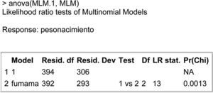
As in the case of the logistic regression, we can calculate the general goodness of fit by comparing the adjusted model (MLM.1) with the null model (adjusted for the independent term) to calculate the general goodness of the fit.

The following code in R allows us to obtain the general goodness of the fit making use of the likelihood ratio test.

Construction of the null model:

Fig. 11 shows the comparison of models based on the likelihood ratio test. The table shows the statistical significance (Pr(Chi) = p-value of the contrast of hypotheses) – thus confirming that globally, the predictor variable smoking mother (smokermother) significantly contributes to the result obtained by the dependent variable (weightbirth).

Figure 11.

Goodness of fit test for the multinomial model.

Acknowledgement

Thanks are due to Pérez-Vicente S. and Rodríguez del Aguila M.M. for their invaluable help and advice.