Simple linear and multivariate regression models

Summary

In biomedical research it is common to find problems in which we wish to relate a response variable to one or more variables capable of describing the behaviour of the former variable by means of mathematical models.

Regression techniques are used to this effect, in which an equation is determined relating the two variables. While such equations can have different forms, linear equations are the most widely used form and are easy to interpret.

The present article describes simple and multiple linear regression models, how they are calculated, and how their applicability assumptions are checked. Illustrative examples are provided, based on the use of the freely accessible R program.

Introduction

One of the main aims in scientific research is to establish relationships among different random variables through the development of models or algorithms. Such relationships are generally difficult to detect. One way to simplify the problem is to establish a model relating a study variable (dependent variable) to a set of predictor variables (independent variables or covariables).

Depending on the intended use of these models, two major groups can be distinguished in qualitative terms: models developed with an explanatory purpose, in which the degree of fit of the variables is not so precise, or predictive models, in which the degree of fit must be optimum.

One of the most widely used procedures for fitting a study variable to a set of covariables is the linear regression model. This is one of the most commonly used techniques in biomedical research. Its versatility, simplicity and easy interpretation define it as one of the most potent tools for determining the existence of a relationship between a studied dependent variable (normally referred to as Y) and one or more independent predictor or explanatory variables referred to as X₁, …, X_n.

The term “regression” refers to the fact that the observed data tend to group around the mean (regression to the mean), while “linear” refers to the type of equation used in the model to determine the relationship between the variables.

Prior definitions

We will introduce the concept of Pearson's linear correlation coefficient, r.^1,2 This is a parameter allowing us to detect a linear correlation between two random variables. The parameter is defined as:

where cov(X, Y) is the covariance or dispersion between the variables X and Y, indicating the sense of the correlation between the two variables (positive or negative); S_x and S_y are the standard deviations of X and Y, respectively.

The correlation coefficient presents a value of between −1 and 1, and indicates the degree of linear association or correlation between the variables X and Y. In this context, values close to 1 indicate a positive linear association, while values close to −1 indicate a negative linear correlation. In turn, a value close to 0 points to the absence of linear correlation – indicating a poor fit of the data points to a straight line. This does not necessarily mean that there is no dependence between the variables, only that any dependence that may exist is not of a linear nature.

The coefficient of determination or R² in turn is the square of Pearson's linear correlation coefficient. It can be interpreted as the percentage variability of the dependent variable explained by the model (independent variable or set of variables). The coefficient of determination varies between 0 (absence of linear correlation) and 1 (exact linear correlation). For models developed with predictive purposes, a coefficient of determination very close to 1 is usually sought (≥0.8).

Instead of the value R², we usually calculate the corrected or adjusted R², which avoids problems of few cases and many variables.

Simple linear regression

The simple regression equation is of the form:

indicating that the dependent variable Y is approximately a linear function of the covariable X, while ¿ measures the degree of discrepancy of this approximation, α is the independent term, and β is the regression coefficient or slope of the straight line. The term ¿ (or perturbation element) refers to the error of approximating the observed value Y by means of the linear estimation obtained from the model.

In this way it is possible to interpret a complex problem, such as the determination of the relationship between two study variables X and Y, as a problem of estimating the parameters α and β.

Eq. (2) can also be expressed as follows:

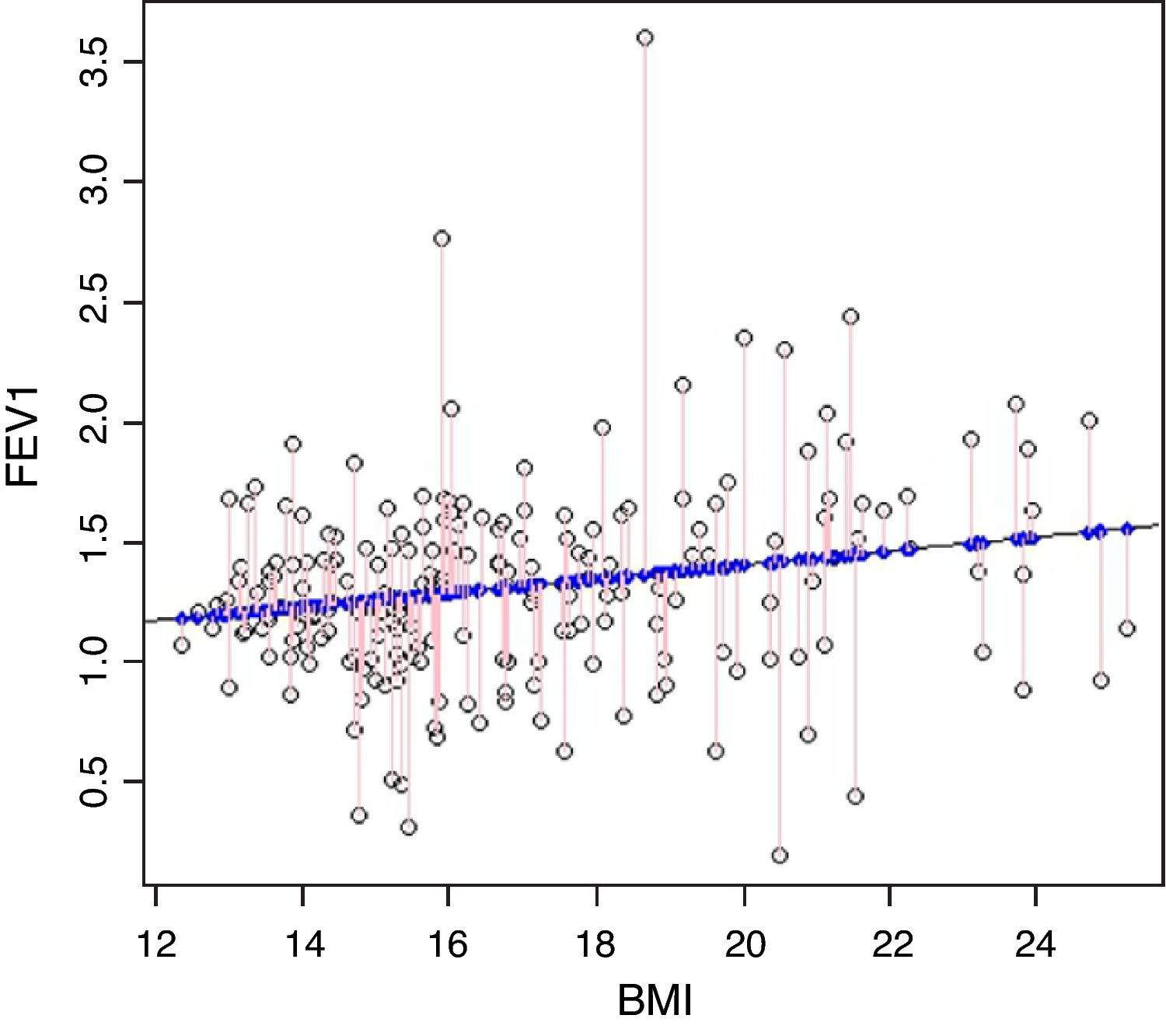
where E[X] is the mean of the variable X. This expression facilitates interpretation of the model, since the independent term, α′, can be seen as the value predicted by the model for the mean value of the covariable (when X = E[X]). In addition, it avoids extrapolation problems (values predicted by the model at points where there are no observed data).

In order to resolve the above equation under optimum conditions, it is necessary to verify a series of hypotheses that will mostly have to be checked on an a posteriori basis. Initially it is recommendable to use a dispersion chart or dot plot³ (Fig. 1) to represent the variables X and Y, allowing us to visually assess the presence or absence of a linear relationship between the two variables.

Figure 1.

Dispersion chart (dot plot) of the variable FEV1 versus BMI, together with the estimated regression straight line. The values from each point to the straight line are the residuals. The tracing is obtained in R with the command plot(fev1 ∼ bmi, data = allergy).

We will address the hypothesis of the model by means of the following example:Suppose we wish to contrast the hypothesis that linear dependency exists between forced expiratory volume in the first second (FEV1) and the body mass index (BMI) in children. In this case we take as dependent variable Y = FEV1, and as independent variable X = BMI, since it is the latter parameter which might explain certain variability in the forced spirometry results obtained.

Hypothesis of the model:

• I.

  The dependent variable Y can be expressed as a linear combination of the independent variable X in the form described in Eq. (2). The coefficients to be determined are assumed to be constant but unknown. Non-applicability of this hypothesis is usually referred to as specification error. In our example, this condition means to say that forced expiratory volume in the first second (FEV1) is proportional to the body mass index (BMI) plus a certain amount.

• II.

  The expected value of the perturbation element ¿ is 0 (the mean of the approximation errors is 0). Non-applicability of this hypothesis introduces noise in the estimation of the independent term α, making its correct interpretation in the model impossible.

• III.

  The dispersion of the approximation errors is constant (homoscedasticity), and the errors are not correlated to each other. Heteroscedasticity tends to occur in cross-sectional studies, where the data analysed come from a number of different populations, while correlation between errors is usually seen in observations extracted over a period of time. As an example, if we have data from two different populations (e.g., a paediatric group and an adult group), it is possible that for one same body mass index the variability of the spirometric results differs between the two populations.

• IV.

  The distribution of errors is due to common causes of variation (they therefore follow a normal distribution with a mean of 0 and constant deviation). This type of condition expresses that the degree of variability of the errors of the approximation of the model is attributable to unknown causes which isolatedly exert very little influence, but which globally produce small variations of the predicted value with respect to the actual or true value.

• V.

  Colinearity in the analysed data. This problem manifests when there is dependence between certain explanatory variables, or when a transformation of the dependent variable as independent variable is being used. An example of this type of error may be when attempting to predict the lung capacity of a given patient from the BMI and weight and height of the patient. The variable BMI is represented in the other two variables, thus introducing colinearity in the model.

• VI.

  The number of observations must be greater than the number of independent variables intervening in the model. In general, a number of 10 observations is estimated per covariable introduced in the model.

Under the above hypotheses, the next step is to obtain the coefficients of Eq. (2) by means of the minimum squares method. This method involves minimisation of the squared distances of each cluster point (observed values) with respect to the estimated point of the regression straight line (predicted or estimated values) (Fig. 1).

In the event the variables X and Y are non-correlated, or the covariance between them is zero, Pearson's correlation coefficient will also be zero, and the regression straight line (2) would be a constant equal to the independent term α.

The sign of the covariance, and thus of Pearson's correlation coefficient, is the sign of the slope of the straight line. Accordingly, a positive linear correlation is given by a positive value of the mentioned coefficient, while a negative correlation is given by a negative coefficient for the slope.

An example has been generated with the R program to illustrate how this analysis is made, and show the type of results obtained.

We read the data from an SPSS file (the foreign library must be loaded in order to read files of this kind), and file them as a series of data called allergy.

>library(foreign)
>allergy<-read.spss(“fileroute”,	use.value.labels = T	max.value.labels = Inf,
to.data.frame = T)

use.value.labels = T implies that we will use the labels defined by the SPSS package as values of the variables.to.data.frame = T implies that the data read from the SPSS package will be filed in a data.frame (the data frames of R are the way in which the mentioned program files a set of variables).

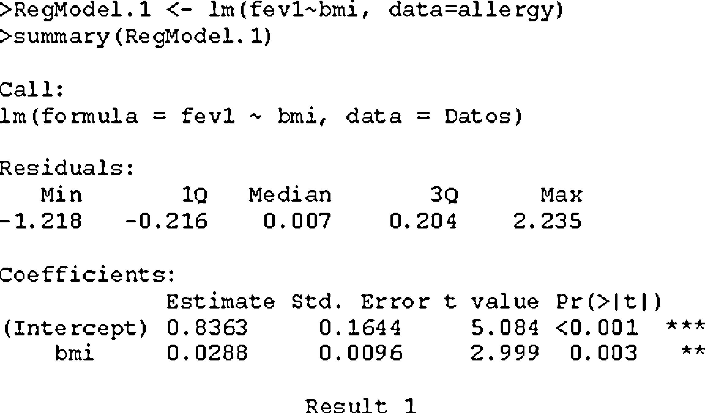
The simple linear regression model (RegModel.1) is defined from the data filed in the allergy file by means of the function lm, which reads a formula with the variables to be fitted and a data set.

We first have the call to the function we have used, followed by a description of the distribution of residuals (difference between the values observed and predicted by the model).

We next have the estimation of the coefficients (intercept = α), standard error, and the value of the statistic associated to the contrast of hypothesis of assuming the coefficient to be 0, together with its p-value as shown in result 1. Lastly, we have the result of applying analysis of variance (ANOVA¹) of the variable FEV1 with respect to the covariable BMI, which checks whether the regression model is globally significant.

In this example both the independent term (α = 0.84, with associated p-value < 0.001) and the coefficient associated to the slope of the straight line appears as significantly non-null (β = 0.03, with associated p-value = 0.003). The linear regression equation therefore would be:

which is interpreted as meaning that for every 1% increase in BMI, the FEV1 values increases an average of about 0.03. The value 0.84 would be the mean FEV1 for bmi = 0. Therefore, in order to avoid the problem of extrapolating scantly realistic values in the model, the latter is adjusted for the centred covariable BMI, applying Eq. (2).

The new variable is defined, subtracting its mean:

>allergy$bmim<-allergy$bmi-mean(allergy$bmi)

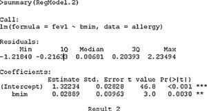
The new model RegModel2 is defined:

>RegModel.2 <- lm(fev1∼bmim, data=allergy)

New statistical summary of the model:

On comparing the initial model with this centralised model, the only element distinguishing them is the independent term of the straight line; even the level of significance is the same (differing minimally due to the rounding errors).

The resulting model would now be as follows:

In this way, the result of a forced spirometry test increases an average of 0.03 times for every 1% increment in BMI with respect to the mean, and 1.32 would be the mean FEV1 value when the BMI is equal to the mean (E[bmi] = 16.82).

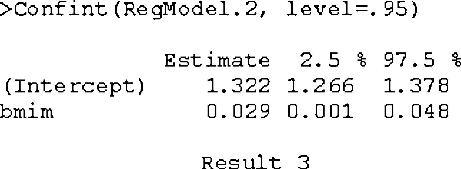
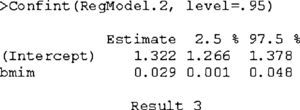
For calculation of the 95% confidence intervals (95%CI) of the coefficients associated to the model, use is made of the Confint expression, the arguments of which are a regression model and a level of significance.

In result 3, the 95% confidence interval for the independent term is (1.266, 1.378), which means that the independent term of the model is between these two values with a certainty or confidence of 95%. Likewise, the slope of the straight line is between 0.001 and 0.048, with a certainty of 95%. In both cases it may be noted that the value 0 is not included within the intervals, which means that the coefficient associated to BMI is non-null at a level of significance of 5%.

Under the conditions of the model, the confidence interval for the slope confirms the contrast of hypothesis for determining the usefulness of the independent variable X (in this case BMI) as an explanatory variable of the independent variable Y (FEV1), and is based on the Student t-statistic which contrasts the hypothesis:

In the case of the simple linear regression, this contrast coincides with the variance analysis applied to the regression model.

Lastly, it should be mentioned that although there is linear dependence between the variables FEV1 and BMI, the percentage variability of the result of the spirometric test explained by the BMI is very poor (this value being given by the R-square or adjusted R²) – in our case 3.8%. Therefore, if we wish to predict spirometry values, we should explore a set of variables in addition to BMI which could better explain the dependent variable.

Multiple linear regression

Multiple linear regression models are a generalisation of simple linear regression in cases where we have more than one independent or predictor variable. The aim of such multiple regression is therefore to explore and quantify the relationship between a numerical dependent variable and one or more qualitative or qualitative predictor variables.

A multiple linear regression model has the following structure:

where Y = dependent or explained variable, X₀, X₁, X₂, …, X_n are independent predictor or explanatory variables, β₀, β₁, β₂, …, β_n are regression coefficients (constants), and ¿ is the error term, with a normal distribution and which contemplates the part not explained by the independent variables.

This model is based on the same assumptions or postulates as those described for simple linear regression, and which will be checked in the following section: independence of predictor variables (non-colinearity), normality of the residuals, linear type relationship, independence between observations, and equal variances (homoscedasticity).

The regression straight line is obtained estimating the coefficients β_i by means of the minimum squares method, i.e., seeking the best linear equation fitting to the data and minimising the distances between each observed value (Y_i) and the value estimated from the straight line (Ŷ_i). In this case, as we have more than one independent variable it is not possible to graphically represent the relationship between them and the dependent variable (only when we have two predictors, with visualisation in a three-dimensional space).

It is advisable for the sample size to be adequate on applying multiple linear regression. Specifically, the recommendation is to have at least 10 cases for each independent variable included in the model. For example, if we consider a model with four predictors, a sample of at least 40 cases would be required.

The steps involved in constructing a multiple regression model are the following:

• Identification of predictor variables

• Construction of the model

• Selection of variables

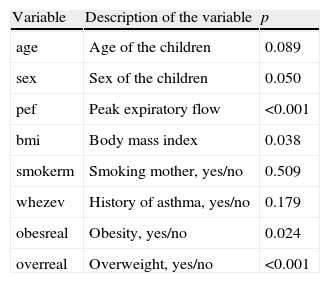
In describing the construction of a multivariate regression model, FEV1 will be used as dependent variable, while the independent or predictor variables will be those shown in Table 1.

Table 1.

Result of applying simple regression analysis to each of the independent variables with respect to the dependent variable FEV1.

Variable	Description of the variable	p
age	Age of the children	0.089
sex	Sex of the children	0.050
pef	Peak expiratory flow	<0.001
bmi	Body mass index	0.038
smokerm	Smoking mother, yes/no	0.509
whezev	History of asthma, yes/no	0.179
obesreal	Obesity, yes/no	0.024
overreal	Overweight, yes/no	<0.001

Identification of predictor variables

The possible predictor variables of the model can be explored in several ways:

• -

  If the independent or predictor variables are quantitative, use is made of correlation analysis based on Pearson's correlation coefficient between the dependent and independent variables, and among the different predictors. This latter analysis in turn makes it possible to detect possible colinearity between variables that must be corrected. Alternatively, we can apply a simple linear regression model for each predictor variable acting as candidate for inclusion in the model, versus the common dependent variable.

• -

  If the independent variables are qualitative, the Student t-test (qualitative with two groups; in this case simple linear regression can also be used) or ANOVA is applied (qualitative with more than two groups) to check the relationship between the dependent variable and the predictor variables.

On applying a simple regression model to each independent variable with respect to the dependent variable FEV1, we obtain the significances shown in Table 1.

Construction of the model

Construction of the model involves estimation of the beta-coefficients to derive the estimated regression equation. The equation is calculated by minimising the squared distances between the observed and predicted values, i.e., min Σ(y_i − ŷ_i)².

The regression coefficients are constant values that affect each explanatory variable, and indicate the change in the dependent variable for each unit increase in the predictor variable adjusted for the remaining variables. In general they are standardised to compare the relative importance of each variable. Such standardisation is carried out by dividing each beta-coefficient by the corresponding standard error. The variable with the greatest standardised coefficient is the variable making the greatest contribution to the regression model.

The ANOVA table offers important information which can be obtained in any multiple regression model. The table reflects the significance of the global regression model; accordingly, when significant (p < 0.05), it indicates that considering linear regression makes sense. Such significance differs from that of each regression coefficient, which is established from the Student t-test. There may be joint significance, but some explanatory variable may not be explanatory.

In some cases the contribution coefficient is calculated, represented by multiplying the correlation coefficient by each of the beta-coefficients obtained. The sum of all of them is equal to R² or the coefficient of determination (square of the multiple linear correlation coefficient).

On the other hand, the standard error of the estimation, i.e., standard deviation of the residuals, indicates variability not explained by the regression model. The obtainment of relatively low values is indicative of a good fit.

Initially it is of interest to include all the variables serving as candidates for inclusion in the model at once or in a single block. This method is usually the first to be used when we have several variables as candidates for inclusion in the regression, since it allows us to see the importance which each variable may have in the constructed model. The selection of variables is seen in the following section.

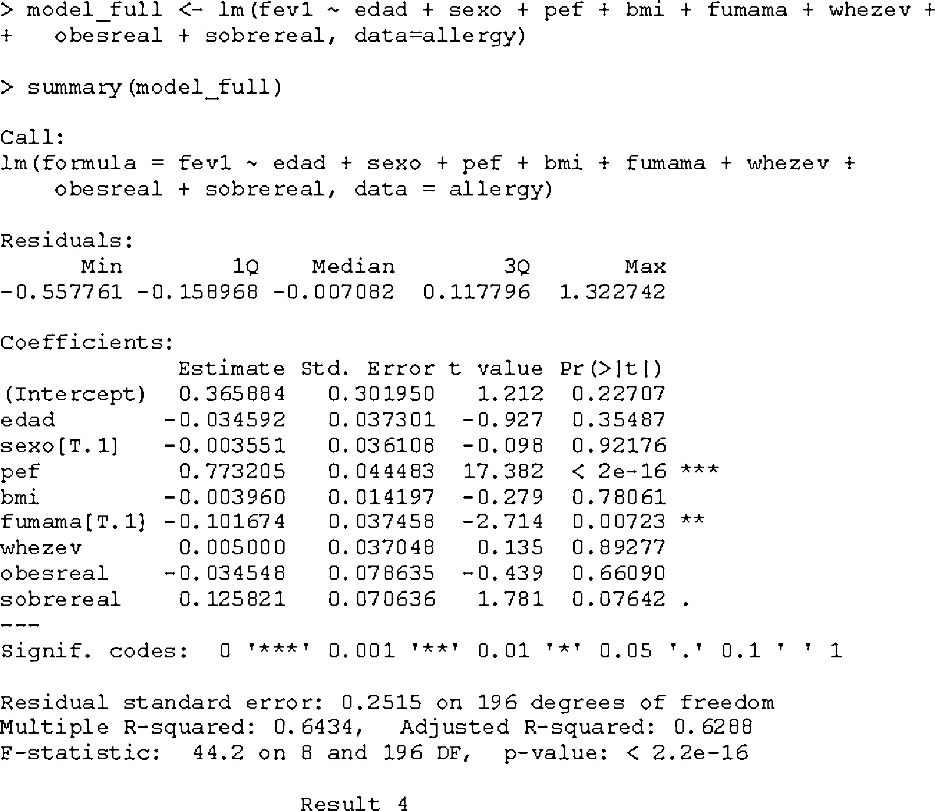
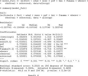
As an example, we apply the multivariate linear regression model in R taking as independent variables all those shown in Table 1 as a single block.

The complete model in result 4 indicates that the variables which are significant at the indicated levels are pef, smokerm and overreal. The ANOVA of the model is significant (p < 0.001), and the adjusted coefficient of determination is 0.629, indicating that 62.9% of FEV1 is explained by all the included variables (both the significant and the non-significant ones). It is advisable to apply a variables selection procedure and eliminate those variables lacking relevance, as will be seen in the section below.

Selection of variables

For the selection of independent variables, whether these are quantitative or qualitative must be distinguished.

• –

  Quantitative variables: these are included as such in the model.

• –

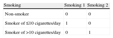
  Qualitative variables: in the case of dichotomic variables it is advisable to homogenise the values, i.e., recode them all to 0 (absence of the risk factor) or 1 (presence of the risk factor). In the case of polychotomic variables, these are to be transformed into dummy variables (as many variables as there are categories, minus 1). As an example, for the variable smoking, recoded as 1 = non-smoker, 2 = smoker of ≤10 cigarettes/day and 3 = smoker of > 10 cigarettes/day, two dummy variables would be required – one termed smoking1, with a value of 1 for category 2 and 0 for the rest (thus representing the smokers of ≤10 cigarettes/day), and smoking2, with a value of 1 for category 3 and 0 for the rest (thus representing the smokers of >10 cigarettes/day) (Table 2). Category 1 serves as reference for both variables (in R the function as.factor automatically converts the numerical variables into qualitative variables).

  Table 2.

  Relationship between a qualitative variable and the dummy variables obtained from it.

  Smoking	Smoking 1	Smoking 2
  Non-smoker	0	0
  Smoker of ≤10 cigarettes/day	1	0
  Smoker of >10 cigarettes/day	0	1

All the dummy variables are to be included in the model even if some of them may not be significant, since they form part of a global variable.

Regarding the way to introduce the independent variables in the model, a number of alternatives are available:

• –

  Introduction method: includes all the predictor variables at once (see ‘Construction of the model’).

• –

  Forward method: starting from a model only with the constant or independent term β₀, followed by progressive introduction of variables in the equation, provided they are significant.

• –

  Backward method: all the variables are initially considered in the model, and those lacking significance are then progressively eliminated.

• –

  Successive steps method: this represents a combination of the above two approaches.

Any of these described methods can be combined in several blocks; for example, a first block can use the introduction method with a series of variables, while a second block can involve the introduction of a different set of variables using the forward method.

The statistical packages incorporate these procedures in the selection of variables, although they are subject to some controversy, since they produce discrepant results.⁴

We can describe the inclusion/exclusion criteria for variables based on the following:

• I.

  Level of significance of the associated coefficient (we generally use values p > 0.1 as exclusion criterion and p < 0.05 as inclusion criterion). A purported drawback of this technique is the fact that it includes variables even if they contribute little information on the general variability of the model.

• II.

  Criteria based on the so-called loss of information function. Within this set of criteria we have the Akaike information criterion (AIC),⁵ which seeks the model that best adjusts to the data with the minimum number of variables possible, thus producing simpler models. In this way covariables are sought that afford a good explanation of the dependent variable, and whose information proves necessary. This technique is based on minimisation of the loss of information function, penalising for the number of variables introduced; in this way the AIC indicator is calculated. We choose the model that minimises the AIC. This is the technique used by the R program.

• III.

  Another way to incorporate variables to the model is to observe the changes experienced by the coefficient of determination R². The value of R² is examined with and without the variable in question, and if the change is significant, the variable will be relevant for inclusion in the model. This is the technique used by the SPSS statistical package.

• IV.

  Calculation of the tolerance values (see section ‘Colinearity’) also helps to detect important variables; accordingly, a high tolerance value (in the order of 1) indicates that the variable is relevant, while a low tolerance value (close to 0) may be indicative of colinearity, and so the mentioned variable would not be relevant.

A particular case of candidate variables for inclusion in the model is represented by interactions usually between pairs of variables.⁶ Interaction is calculated as a product of predictor variables, generally one quantitative variable and one qualitative variable, and it identifies the fact that the levels of the first variable differ as a function of the levels of the second variable. In the regression models they are introduced as any another variable, taking into account that if interaction is included, the two independent variables conforming it must be included.

These techniques for the selection of variables are simply statistical tools that help in the decision process, though in no case should they substitute clinical criteria when it comes to selecting variables that may be correlated or be of relevance for consideration.

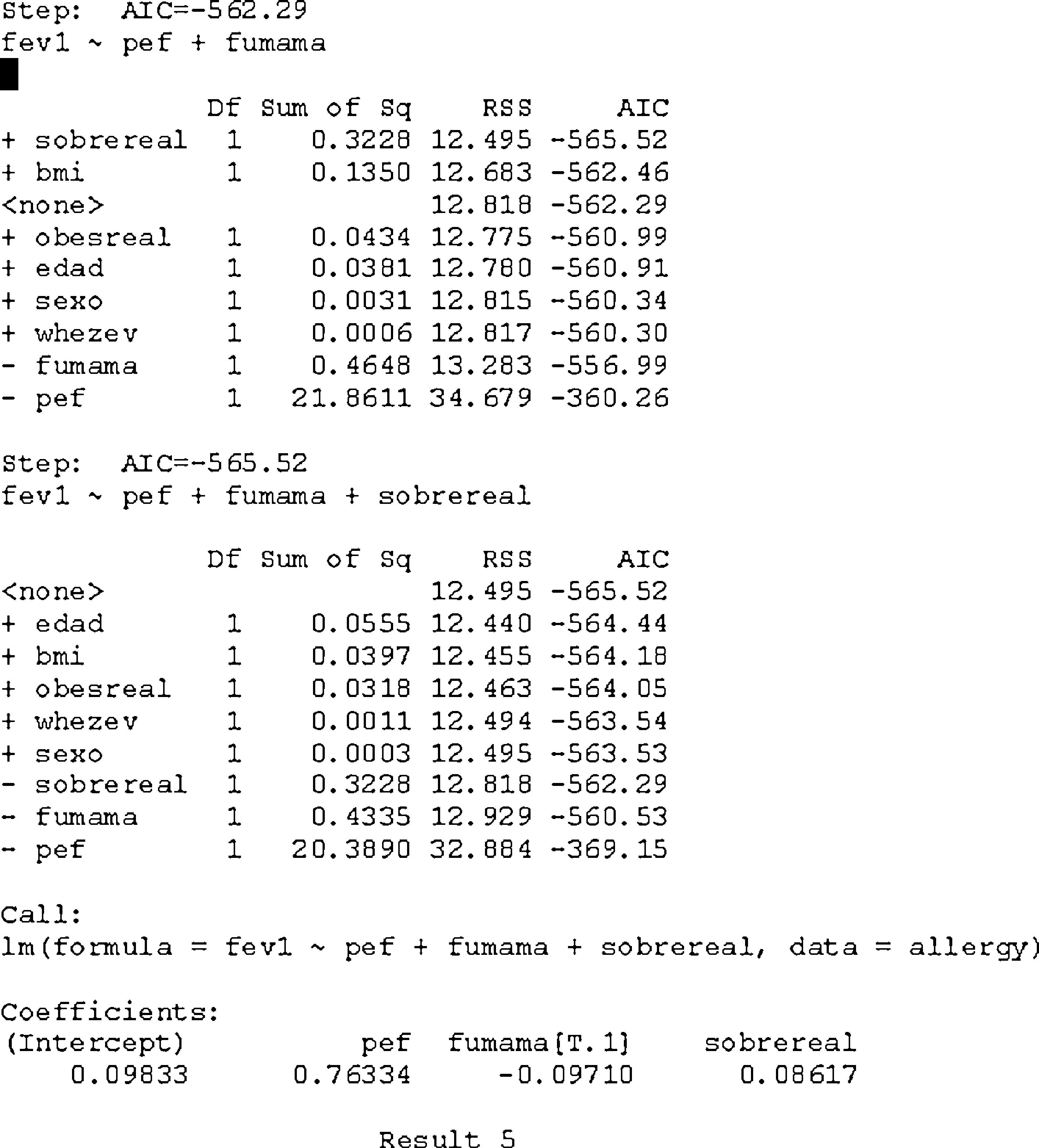
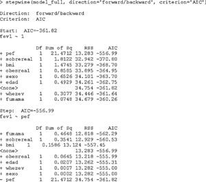
To illustrate the selection of variables, the AIC selection criterion is shown below in the R program, combined with a successive steps procedure. Previously a full model such as that described in the above section must have been developed.

As we seen in result 5, we initially start with a model with the independent term; in the subsequent steps we evaluate the inclusion of each of the candidate variables that are not in the previous model (indicated with the sign +), or exclude those of lesser relevance for the model (indicated with the sign −). The process is completed when the loss of information function cannot be improved (minimum AIC).

Final model:

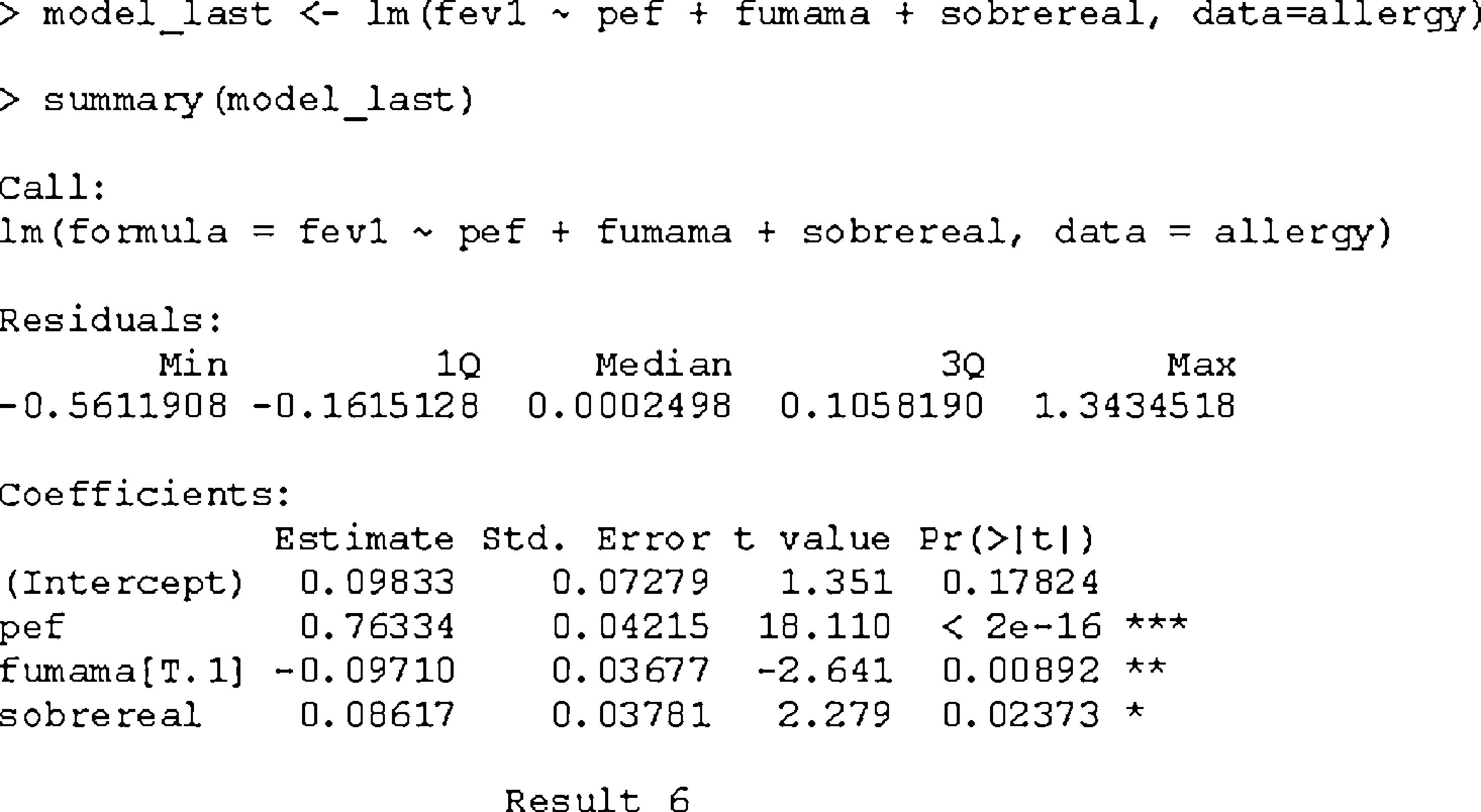
Interpretation: for each unit increase in the value of pef, the FEV1 value increases an average of 0.76334, adjusting for the remaining variables. In the case of a smoking mother (smokerm = 1), the FEV1 value decreases an average of 0.0971 units, likewise adjusting for the remaining variables. Overweight status in turn increases the FEV1 value an average of 0.08617 units. The final model is shown below with the significances and R² value, which in this case is 63.5%.

The variable smokerm[T.1] in result 6 is a factor variable with two possible values: 0 = non-smoker, 1 = smoker. We take the value not in brackets (non-smoker) as reference category. The value of pef should have centred with respect to its mean in order to be able to interpret the independent term, but this is less relevant in multivariate regression procedures than in simple regression.

Goodness of fit

Once the model has been constructed, it might not be definite, since checking is required of the assumptions or postulates for applying the linear regression model – a task that always must be done on an a posteriori basis. Goodness of fit involves evaluating each of the characteristics described below. If any of them are not verified, alternatives are proposed in an attempt to correct the deficiency. In general, checking of the assumptions is made graphically; as a result, in some cases interpretation is subjective:

• Normality and atypical observations (outliers)

• Linearity

• Homoscedasticity

• Autocorrelation

• Colinearity

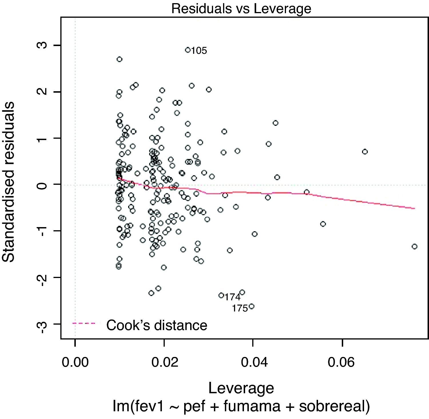
• Influencing observations

Checking of the colinearity assumption only makes sense for multiple regression.

Normality and atypical observations (outliers)

Normality in regression is necessary in order to estimate and calculate the confidence intervals, since otherwise the minimum squared coefficients are no longer efficient. A lack of normality is sometimes attributable to extreme observations.

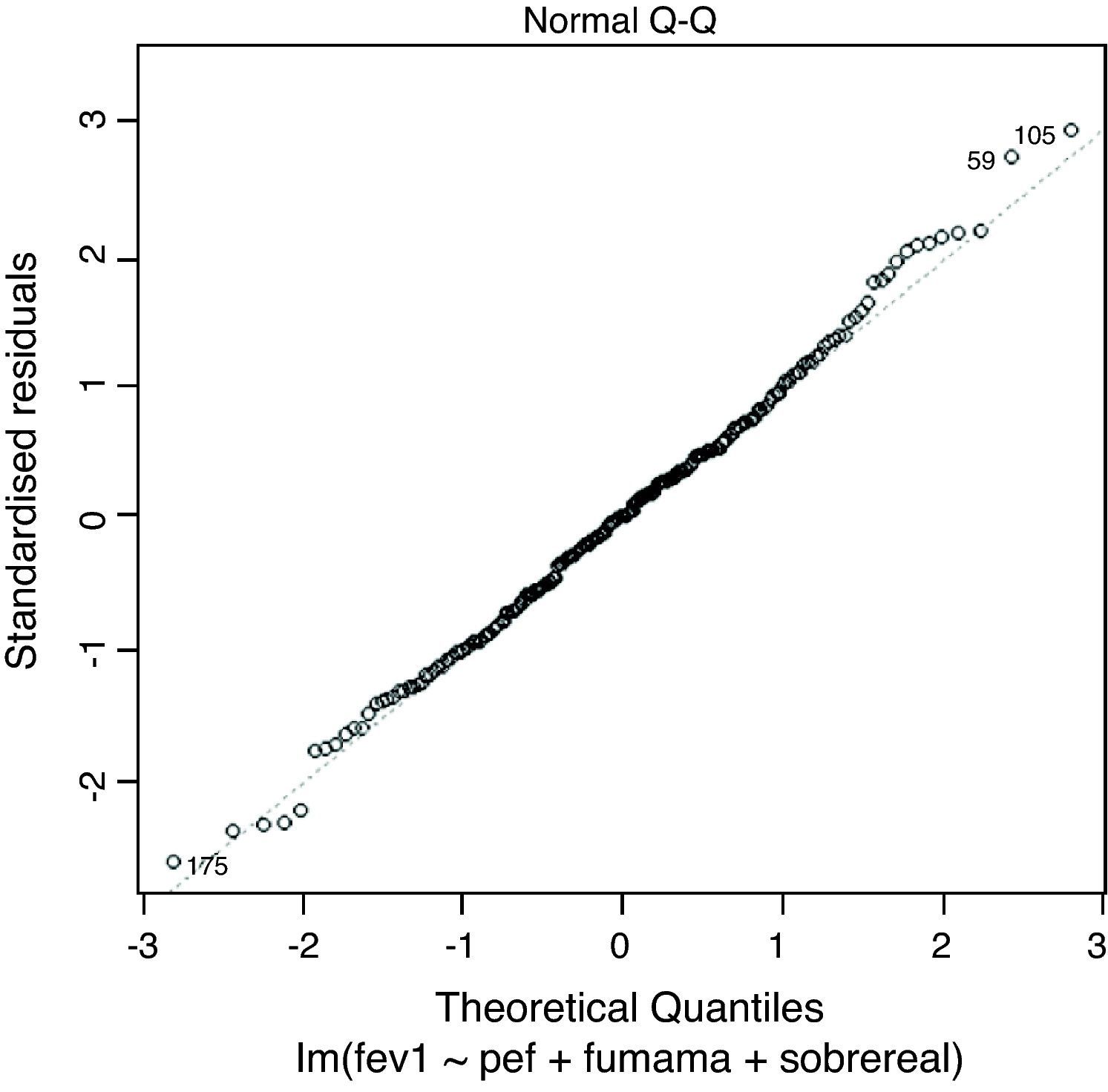
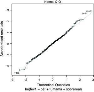
Normality can be checked by the residuals normality plot (diagonal line in the figure). Deviation of the graphical representation from the diagonal line means that the normality assumption is not met (Fig. 2).

Figure 2.

Q–Q figure. The dot plot over the diagonal indicates both linear relationship and normality of the residuals. The tracing is obtained in R with the command plot(model_last2).

Solution for lack of normality:

• –

  Transformation of the dependent variable^7,8 (square root, logarithm, etc.). This change must be taken into account for final interpretation of the model.

• –

  Determination of the influence of atypical values controlled by the response variable/s, i.e., atypical values for each given set of values of the response variable.

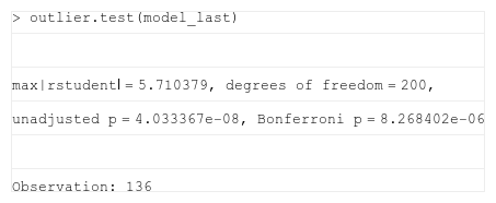
For determining atypical values (outliers) it is common to use standardised residual errors or Student-transformed residual errors. The R program offers a function that performs this process.

> outlier.test(model_last)

max|rstudent| = 5.710379, degrees of freedom = 200,

unadjusted p = 4.033367e−08, Bonferroni p = 8.268402e−06

Observation: 136

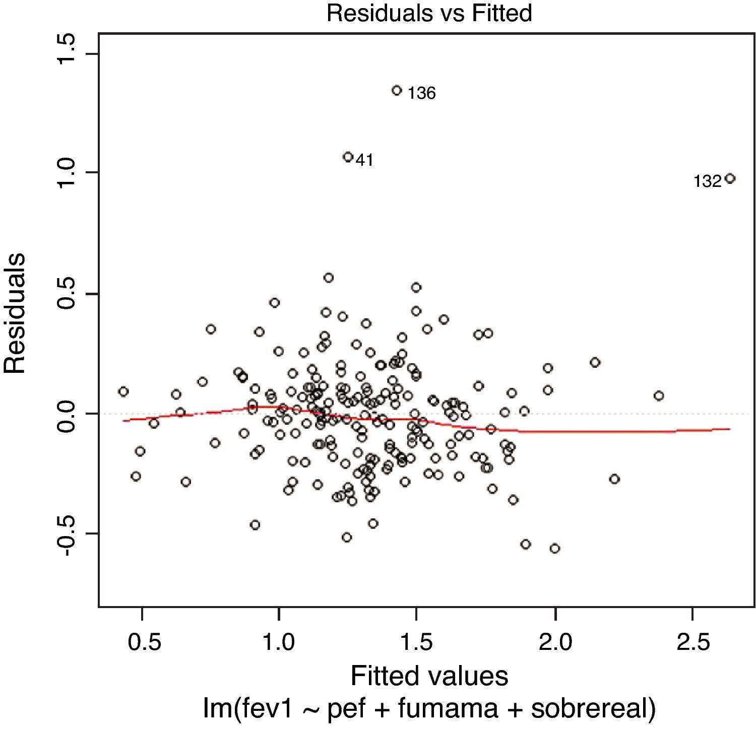
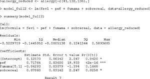
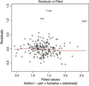
On applying the test that detects anomalous observations or outliers, we find that observation 136 is significantly removed from the rest. However, on examining Fig. 3 we identify another two observations (41 and 132) that also deviate from the rest, even though significance is not reached in this case. Accordingly, they are excluded from the model for the successive checks. The model with elimination of the three observations is again reproduced in result 7.

Figure 3.

Dispersion chart of the adjusted values with respect to the residuals. Of note are the three atypical observations that are removed from the rest. The tracing is obtained in R with the command plot(model_last).

On eliminating the three observations, the variable smokerm loses significance, but we keep it in the model, since it was initially included in the latter. The coefficient of determination R² is now seen to be 67.8%, whereby we gain in terms of explained variability. The rest of the checks or verifications are made on this model, with the elimination of three cases.

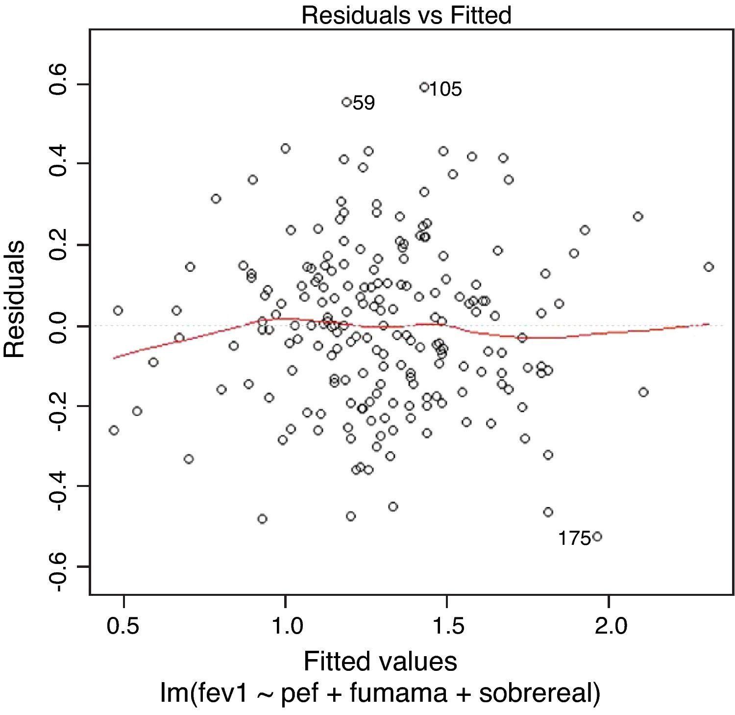
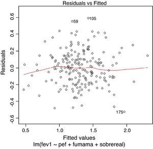
Linearity

In order to check whether the regression model is truly linear, we produce a dispersion chart between the predicted variable or predicted values ŷ_i on the abscissa versus the residuals (y_i-ŷ_i) on the ordinate (Figs. 3 and 4). This tracing must represent randomness in the fit; as a result, if there is some type of tendency or trend, the model will be nonlinear. Another way to observe linearity is by means of the Q–Q plot, where the residuals are represented on the diagonal line of the figure. If this line coincides with the diagonal, the fit is linear (Fig. 2).

Figure 4.

Adjusted values with respect to residuals for the model with exclusion of the three atypical cases. The tracing is obtained in R with the command plot(model_last2).

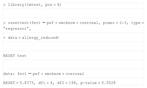
There are specific hypothesis tests that contrast the linearity or nonlinearity of the model, such as the Ramsey RESET test.⁹ This test evaluates the possibility that the dependent variable is a quadratic (Y depends on X²) or even cubic function (Y depends on X³) of the covariable/s, using different methods.

One of the following two options is usually applied to solve the lack of linearity:

• -

  Include predictor variable squared or even raised to the third power.

• -

  Transform predictor variable according to the form or shape of the plot between residuals and the predictor variable.

The result of applying the RESET test with the R program to the model we are adjusting is shown below.

> library(lmtest, pos = 4)

> resettest(fev1 ∼ pef + smokerm + overreal, power = 2:3, type = “regressor”,

+ data = allergy_reduced)

RESET test

data: fev1 ∼ pef + smokerm + overreal

RESET = 0.8375, df1 = 4, df2 = 194, p-value = 0.5028

In this hypothesis test we check whether there may be a quadratic and cubic component in the model, which on yielding a significance of over 0.05 would indicate that the linear fit is adequate.

Homoscedasticity

Homoscedasticity or equality of variances is a condition for applying a linear regression model, and implies that the values of the residuals have homogeneous variance for each value of the independent variable. Consequently, heteroscedasticity (or a lack of homoscedasticity) is an undesirable condition in linear regression, and we must avoid situations such as those seen in Fig. 3, where the residuals increase as the independent variable grows.

In order to detect a lack of homoscedasticity, we again use the above mentioned figure representing the predicted values ŷ_i on the abscissa versus the residuals (y_i − ŷ_i) on the ordinate (Fig. 4). In order to identify which is the variable responsible for the lack of homoscedasticity, we plot each predictor variable versus the residuals, and that variable producing the mentioned lack of homogeneity would be the cause.

Another way to check the homogeneity of variances is the Breusch–Pagan test,^10,11 which contrasts the hypothesis of dependence of the variance of the residuals with the values of the independent variables of the model. The null hypothesis of the Breusch–Pagan test assumes homoscedasticity versus the alternative hypothesis, which admits a certain function of the independent variables in the behaviour of variation of the residuals.

Solution:

• –

  The most widely used method for securing homoscedasticity involves transformation of the dependent variable, applying one of the above described functions: logarithm, square root, inverse, etc. (logarithm application usually minimises multiplicative-type heteroscedasticity, while models more oriented towards the analysis of time series are used to extract information on the absence of a common variance in the sample).

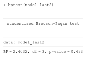
On applying the Breusch–Pagan test in the R program to the adjusted model:

> bptest(model_last2)

studentized Breusch-Pagan test

data: model_last2

BP = 2.4032, df = 3, p-value = 0.493

we obtain a significance of 0.493. The null hypothesis of homoscedasticity is thus accepted. (On applying this test to the full database which includes the three atypical observations or outliers, heteroscedasticity is obtained.)

Autocorrelation

Another assumption or postulate that must be checked by the linear regression model is the absence of autocorrelation, i.e., there must be independence among the residuals. Autocorrelation occurs when there is similarity among the observations as a function of time, and as such it therefore constitutes a mathematical tool to detect certain patterns among patients.

In order to detect autocorrelation we usually apply the Durbin–Watson¹² (d) contrast, and depending on the results obtained, we can have three levels of autocorrelation:

• –

  If 0 < d < 1.5: positive autocorrelation

• –

  If 1.5 < d < 2.5: no autocorrelation

• –

  If 2.5 < d < 4: negative autocorrelation

Thus, the ideal situation is to obtain a result for this test of between 1.5 and 2.5.

Application of this hypothesis test makes sense when the data show a certain ordering in time and space; it is very important not to order the database by any other variable.

If autocorrelation is observed it is because the independent variables are not adequately explaining the behaviour of the dependent variable; as a result, the error term ¿ in Eq. (2) would incorporate this tendency.

Solution:

• –

  Conduct a study of the observations by means of the time series method instead of linear regression.

• –

  Calculate the difference between consecutive observations.

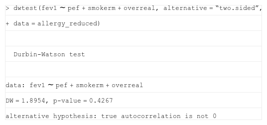
The Durbin–Watson test applied in the R program would be as follows:

> dwtest(fev1 ∼ pef + smokerm + overreal, alternative = “two.sided”,

+ data = allergy_reduced)

Durbin-Watson test

data: fev1 ∼ pef + smokerm + overreal

DW = 1.8954, p-value = 0.4267

alternative hypothesis: true autocorrelation is not 0

The value of the Durbin–Watson test is 1.89, which is located in the interval in which no autocorrelation is considered to exist. This is moreover confirmed by the hypothesis test, which contrasts the absence of autocorrelation as null hypothesis (p = 0.4267)

Colinearity

Colinearity or multi-colinearity¹³ is the dependence existing between predictor variables. This occurs when we have collected a large number of variables in the study that are correlated among each other and are included in the model as predictors. Colinearity also increases with the inclusion of interactions among variables.

Colinearity likewise constitutes an undesirable situation in the context of multiple regression, since it increases the variability of the coefficients – the estimations thus becoming very unstable. Colinearity is detected in the following ways:

• –

  High coefficient of determination values R² and non-significant regression coefficients.

• –

  High and significant correlation coefficients between explanatory variables.

• –

  Tolerance/inflation factor of the variance. The tolerance of an independent variable is the part of the variable not associated to other predictor variables. If a variable has a tolerance of 0.10, for example, it means that the variable shares 90% of its variability with the rest of variables, and therefore would represent a redundant variable. The inflation factor of the variance is calculated as 1/tolerance. Thus, for a variable it is desirable to obtain high tolerance values and, in contrast, to obtain low inflation factors of the variance. As a general criterion it may be affirmed that a tolerance of less than 0.10 is indicative of multi-colinearity.

Solution:

• –

  Eliminate the predictor variable causing colinearity.

• –

  Perform a principal components analysis to reduce the dimensionality of the problem. This analysis involves reducing the number of independent variables in the study, representing them by means of a smaller number of factors, so that each factor reflects those variables that are inter-related. These factors in turn are non-correlated among each other (i.e., they present zero correlation).

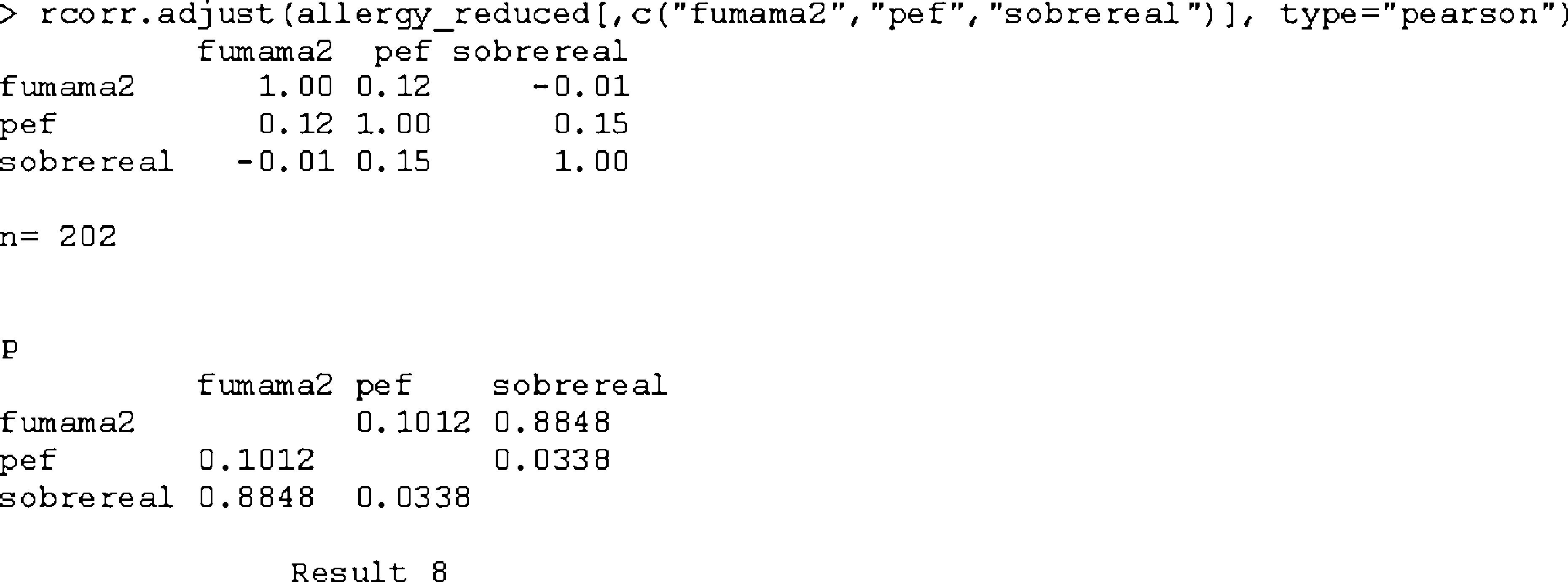
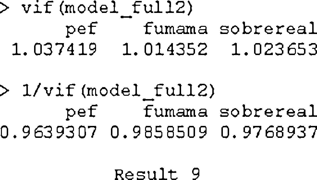
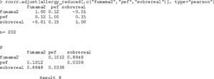
The R program calculates the Pearson correlation coefficients among the independent variables, as well as tolerance and the inflation factor of the variance as shown in results 8 and 9.

The Pearson correlation coefficients indicate that they are not significant.

The tolerance values of the three variables in result 9 indicate the non-existence of colinearity, as the values are close to unity.

Influencing observations

When we graphically represent the dispersion chart in the case of multiple regression, a series of observations sometimes appear separated from the rest of the sample. These observations may be atypical or influencing.¹⁴ In the first case they appear separated from the rest of the observations of the dispersion chart (section ‘Normality and atypical observation’), while in the second case we have observations that could be influencing the estimation of the model (the regression straight line slope would change).

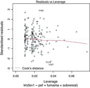
The way of detecting the influencing observations is by means of the dfbetas, or change produced in the regression coefficients on eliminating the possible influencing observation. In order not to consider these values as influencing points, the dfbetas must be less than 2/√n, where n is the size of the sample. Another way to check influencing observations is by examining the Cook distance, which must be <1.

Solution:

• –

  Review the data before eliminating.

• –

  Determine whether they represent a subpopulation, and if there are several, include a variable that differentiates them from the rest.

The R program checks the existence of influencing observations by means of Fig. 5. The values appearing outside the dotted band would be influencing observations.

Figure 5.

Cook distances plot. The points outside the dotted band are considered to be influencing observations. The tracing is obtained in R with the command plot(model_last2).

Validation of the model

Once the regression model has been constructed and the application assumptions or postulates have been checked, the last step is to validate the model. Validation is a way of giving final approval of the model, in the sense that it can be used for predictive purposes.

There are several ways for validation:

• –

  Including new cases and checking the similarity between the observed values and those predicted by the model.

• –

  Cross-validation: one-half of the cases are taken for construction of the model (training group) and prediction is made with the other half – likewise checking the similarity between the two groups.

• –

  Leave one out: adjustment is made with n-1 cases, and validation is made with the remaining case. In this way we can perform as many validations as there is sample size. Validation is carried out by checking that the multiple correlation coefficients in both cases are similar.

Prediction

A frequent application of linear models is to obtain values predicted by the model in relation to data different from those observed in the study. In order to guarantee the representativeness of these values, the following conditions must be checked:

• –

  The model fits well to the observed data. This condition can be checked with the adjusted R², which depending on the situation will be required to be more or less close to 1. For example, if we wish to carry out a study to validate the use of a given drug, we would require a very high adjusted R². In contrast, if we wish to analyse factors which may lessen the quality of a certain medical process, an adjusted R² of 0.8 might suffice.

• –

  The model has been validated.

• –

  Extrapolation problems. The predictions made by the model are valid in the range of the observed covariable values. We must choose a combination of values of the explanatory variables that make sense in our sample.

In our example we see that R² is 0.6782, which means that 67.8% of the variability of the data is explained by the covariables. This R² perhaps would not suffice to accept the model for predictive purposes, and we would have to use some additional variable. Lastly, if we take covariable values that are plausible in our study, such as for example (pef = 1.0, smokerm = 1 and overreal = 0), indicating that a patient with pef = 1, a smoking mother and no excess body weight, the model would predict a mean FEV1 of:

In the same way, we can calculate as many predicted values as there are combinations of the covariables within the study range.

Final note

All the statistical analyses in this article have been made with the freely distributed R program.¹⁵

For data reading from SPSS files, use has been made of the foreign library.¹⁶