Los eventos climáticos extremos pueden tener consecuencias graves en la población y el medio ambiente, por lo que en este artículo para la ciudad de Mexicali, México, con una serie de tiempo de 1950 a 2010, se analizan las tendencias anuales de temperaturas extremas; asimismo, se estiman los periodos de retorno de 5 a 100 años mediante la modelación de la temperatura máxima estival y la temperatura mínima invernal. Para determinar las tendencias temporales se aplicaron la prueba no paramétrica tau de Kendall y el estimador de pendiente de Sen. También se aplicaron la distribución generalizada de valores extremos (GVE) a la aproximación de máximo por bloques, y la distribución generalizada de Pareto (DGP) a valores sobre un umbral determinado previamente. Debido a las características no estacionarias de la serie de valores de temperatura, se incluyó la tendencia temporal como covariable en el parámetro de ubicación, observándose mejoras sustanciales, sobre todo respecto a la temperatura mínima extrema en comparación con lo obtenido con la distribución GVE sin covariable y con la DGP. Se encontró una tendencia positiva estadísticamente significativa para ambas temperaturas extremas: máxima estival y mínima invernal. Hacia finales del siglo XXI la temperatura máxima extrema podría ser de 2 a 3 °C más alta que la actual, y el invierno podría ser menos severo, ya que el modelo probabilístico sugiere incrementos de 7 a 9 °C en la temperatura mínima extrema respecto del periodo de base estudiado. Se analizan las posibles consecuencias de lo anterior en la ciudad de Mexicali.
Extreme weather events can have severe consequences for the population and the environment. Therefore, in this study a temporal trend of annual temperatures was built with a time series from 1950 to 2010 for Mexicali, Mexico, and estimates of 5- to 100-year return periods are provided by modeling of summer maximum and winter minimum temperatures. A non-parametric Kendall’s tau test and the Sen’s slope estimator were used to compute trends. The generalized extreme value (GEV) distribution was applied to the approximation of block maxima and the generalized Pareto distribution (GPD) to values over a predetermined threshold. Due to the non-stationary characteristic of the series of temperature values, the temporal trend was included as a covariable in the location parameter and substantial improvements were observed, particularly with the extreme minimum temperature, compared to that obtained with the GEV with no covariable and with the GPD. A positive and significant statistically trend in both summer maximum temperature and winter minimum temperature was found. By the end of 21st century the extreme maximum temperature could be 2 to 3 °C higher than current, and the winter could be less severe, as the probabilistic model suggests increases of 7 to 9 °C in the extreme minimum temperature with respect to the base period. The foreseeable consequences on Mexicali city are discussed.
Various studies have indicated that changes in the frequency and intensity of extreme climate events, such as heat waves, droughts, and foods, can be expected in several parts of the world due to global climate change (IPCC, 2007). Changes in these extreme events are particularly important for society and the environment because, by definition, they occur outside the usual range of adaptability; therefore, they can have severe impacts and significant negative economic effects (Kharin et al., 2007). Variations in temperature extremes are of particular importance due to their relationship to biodiversity and human thermal comfort, as well as their use in climate variability and climate change impact assessments in sectors such as agriculture and energy demand. In the period from 1906 to 2005, the increase in average terrestrial temperature was estimated at 0.74 ± 0.18 °C, and although the value is small, visible effects were observed on many physical and biological systems (IPCC, 2007). According to some projections, extreme heat and cold events may increase during this century, resulting in increased mortality (Curriero et al., 2002; Qian and Lin, 2004).
Studies related to the analysis and modeling of extreme climate events use general circulation models (GCMs) and the extreme value theory (EVT) as essential tools. In particular, EVT models the behavior of extreme observations, i.e., maxima or minima. Its application to climate studies is recent (Naveau et al., 2005), but studies are increasingly using EVT for events related to weather and climate and their impacts on human society and ecosystems (Dixon et al., 2005; Katz et al., 2005; Unkaševiæ and Tošiæ, 2009; Furió and Meneu, 2011; Constantino, 2011; García-Cueto and Santillán, 2012).
Mexico is vulnerable to the climate change phenomenon, but the impacts may not be uniformly distributed. The IPCC (2007) has shown that water shortages will be exacerbated due to temperature increases and reduced precipitation in the northern Mexico and southern United States regions. According to national climate scenarios, the greatest increases in the average annual temperature in Mexico will occur in the northern part of the country, with greater increases in the northwest than in the northeast (Magaña et al., 2012). Increases for the period 2070-2099 will be approximately 3.5 °C in the northwest and approximately 3 °C in the northeast, under the A2 scenario. Tejeda-Martínez et al. (2008) estimated future scenarios for the extreme maximum temperature during the month of July in Mexico. They found that changes in the extreme maximum temperature, compared with the 1961-1990 baseline period, varied from +0.5 °C in the 2020s to +9 °C in the 2050s; the extreme minimum temperature varied between +0.5 ° C in the 2020s and +7 ° C in the 2050s. The increases depended on socioeconomic development and the region of the country.
Extreme temperature studies in Mexico have shown that in the last decades of the 20th century (post-1970), there was a significantly higher rate of increase in maximum temperatures than for minimum temperatures, with contrasting trends between northwestern and central Mexico compared with the rest of the country (Englehart and Douglas, 2005; Pavía et al., 2008; Gutiérrez-Ruacho et al., 2010). Regional analyses, such as those conducted by Herrera (2011) for the state of Nuevo León, Vázquez-Aguirre et al. (2008) for the state of Veracruz, and Peralta-Hernández et al. (2009) for southern Mexico, found a significant upward trend in maximum temperature and the frequency of hot days. In the city of Mexicali, Baja California, García-Cueto et al. (2010) found that there are currently 2.3 times as many heat waves compared with the early 1970s, and both their duration and intensity have increased. Regarding minimum temperatures, Weiss and Overpeck (2005) reported an increase in the duration of the frost-free period in the northern Sonoran Desert, although the frost-free period also shortened in the extreme southeast of this desert. For the Laguna District, significant negative trends were also reported for the monthly minimum temperature (Inzunza-López et al., 2011). Only the study by Ríos-Alejandro (2011) applied EVT to model minimum winter temperatures in the city of Monterrey, Nuevo León, using the Gumbel distribution, and estimated some return periods.
The above discussion confirms that studies conducted at the regional level in Mexico have focused predominantly on studying trends in temperature extremes. The evidence of changes depends on the region considered, the method of analysis, and the available data period. It is clear that with an increasingly urban population, people, infrastructure, and urban ecosystems will become more vulnerable to extreme temperature events due to the limited number of prospective extreme climate events studies. Therefore, the purpose of the present study is to apply EVT to the maximum and minimum temperatures of Mexicali, Mexico and to estimate the return values in periods of 5 to 100 years under the premise that the expected climate in the twenty-first century is non-stationary as a result of anthropogenic forcing, either by an increased greenhouse effect or a change in albedo due to land use changes. This study is important given the vulnerability to extreme temperature events shown on multiple occasions in Mexicali. The construction of these scenarios will be of great importance as an input for researchers who study impacts and for local governments to propose adaptation measures that improve urban resilience.
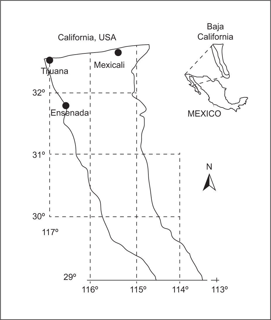
2Area of studyThe city of Mexicali is located in northeastern Baja California, Mexico, at 32.55° N, 115.47° W and 4 meters above sea level. It borders California, USA to the north (Fig. 1). Mexicali has a dry, arid climate with winter rainfall and wide annual oscillation of mean temperatures (BW(h’)hs(x’) according to the García [1988] climate classification). To this climate description can be added that Mexicali has one of the most extreme climates in Mexico, with average July high temperatures of 42.2 °C, and average January highs of 21.1 °C. Mexicali receives 90% of the potential daylight hours each year, and on average 75mm of rain annually. On July 28, 1995, Mexicali reached its all-time high temperature of 52 °C, and on January 13, 1963 its all-time low temperature of −7.0 °C (García-Cueto and Santillán-Soto, 2012).
3DataWe used daily maximum and minimum temperature data from the Mexicali meteorological station. Data were obtained from the records of the Comisión Nacional del Agua (CNA, National Water Commission). Most of the historical information is digitized in the ERIC (Extractor Rápido de Información Climatológica [Rapid Extractor of Climate Data]) V2.0 compact disc. These data, however, had not undergone strict quality control. When large time gaps (which in some cases consisted of several years) were found, the primary sources for these data, including handwritten daily records, were consulted from the original archives. Following this approach, a complete climatological baseline from 1950 to 2010 was developed. Two periods were selected for analysis: summer months from June 1 to September 30, and winter months from November 1 to February 28. This study considered the following: (a) annual maximum and minimum temperature extremes, (b) daily maximum and minimum values of temperature for the selected period. The first consideration leads to the application of the block maxima statistical approach and the second to a threshold value approach. Respect to quality control (QC) data, software RClimdex (1.0) was used (Zhang and Yang, 2004). The main purpose of this QC procedure was to identify errors in data processing, such as: (i) errors in manual keying, (ii) verifying that maximum temperature always exceeded minimum temperature for every calendar day, (iii) identifying data values as outliers in daily maximum and minimum temperature (these values were over four standard deviations (σ) and flagged as potential errors). Daily temperature values were manually checked and edited case by case. Only those values that were confirmed to be erroneous were set to missing and deleted from further analysis. This process of removing inhomogeneous data from the analysis reduced the amount of records originally available. To summarize, of the 16 653 records checked only 10 suspected as erroneous were identified, meaning 0.06% of the whole. These values were checked one-by-one from the original archives and five of them were validated and retained in the dataset as true values; the remaining five were converted to missing values.
A homogeneity test with the RHtest V3 software (Wang and Feng, 2010) was applied to identify possible change points or structural changes in the annual extreme data series of maximum and minimum temperatures. The homogeneity test is based on a two-phase regression model with a linear trend for the entire series. This test identified one change point in the maximum temperature in 1989, and two change points in the minimum temperature, the first in 1977, and the second in 1991. Unfortunately, we did not have the station history metadata, so it is not possible to document the origin of these changes. The last change is likely to be due to relocation of the station according to the weather station chief of Mexicali. The new location is 50 m away from the previous one, without any change in altitude. In the current study, no attempt was made to adjust the maximum and minimum temperature series, because regardless of an artificial change in the recorded values in this weather station, positive temporal trends of temperature have appeared at regional level (García-Cueto et al., 2009).
4Methodology4.1Temperature temporal trendsPrior to the implementation of EVT, a temporal analysis was performed on the series of annual values of extreme maximum temperatures during summer, and extreme minimum temperatures during winter. As both extreme temperatures do not follow a Gaussian distribution, an estimation of monotonous increasing or decreasing trend by simple linear least squares do not seem appropriate. Therefore, we used a non-parametric Kendall’s tau test (Kτ-T) and the Sen’s slope estimator to compute trends (Sen, 1968). The Kτ-T is suitable for cases with monotonous trends and no-seasonal or other cycles in the data. One advantage of this test is that the data need no adjust to any particular distribution. Another advantage of the test is its low sensitivity to abrupt breaks due to inhomogeneous time series (Tabari et al., 2011; Drápela and Drápelová, 2011). Sen’s method uses a linear model to estimate the slope of the trend (Salmi et al., 2002).
For analyzing statistically the extreme values of temperature, two approaches were used: annual block maxima with the utilization of the generalized extreme value distribution and daily values above a threshold with the generalized Pareto distribution.
4.2The generalized extreme value distribution (GEV)Let X1,..., Xn be a sequence of independent random variables with a common distribution function F, and let Mn = max{X1,..., Xn}. The Xi usually represent maximum (or minimum) values measured on a regular time scale, or blocks of time, so that Mn represents the extreme values of the process in n observed time units. For these data, and after linear renormalizing, Mn distributions are given by the generalized extreme value family in the following format:
where (−∞ < µ < ∞), σ > 0, and (−∞ < ξ < ∞) are the parameters of location, scale, and shape, respectively, and x+ = max(x, 0). The type of extreme distribution is determined by the sign of ξ; ξ < 0 corresponds to the Weibull distribution, ξ = 0 to the Gumbel distribution, and ξ > 0 to the Fréchet distribution. The value of î determines the behavior of the tail of the distribution. If ξ < 0, a distribution with a defined upper limit is obtained, while ξ > 0 corresponds to an increasingly upper tail.
To apply GEV distribution to annual minimum temperatures, the usual method for maximum values was applied, but the data were transformed by taking the negative value of those minimum values, i.e., min(x1,...,xn) = −max(−x1,...,xn).
4.3The generalized Pareto distribution (GPD)Because the approximation given by Eq. (1) only takes into account the maximum or minimum values of a time series, many data are omitted. In contrast, the approximation of peaks over threshold (POT) analyzes the values that exceed the threshold value, and the data above this value can be asymptotically approximated by the GPD:
where x−u>0,1+ξ(x−u)/σ˜;>0 and σ˜;=σ+ξ(u−μ). Eq. (2) provides the cumulative probability that X exceeds the value of x, given that it already exceeds the threshold value of u (i.e., Pr [X > x | X > u]). The duality between the GEV and GPD means that the shape parameter ξ is the dominant parameter and commonly determines the qualitative behavior of both distributions. Moreover, the value of σ˜; is found to be dependent on the threshold value, except where the model has the limit value of ξ = 0. The selection of the threshold value is critical to the analysis of the POT approximation. A large threshold value would exclude too much data, leading to a high variance of the estimator; a very small threshold value would likely violate the asymptotic basis of the model, leading to bias (Coles, 2003). In the present study, mean excess function methods were used as a starting point, and the stability assessment of parameter estimators was used for selecting the threshold value, based on adjusting the GPD by postulating a range of different u thresholds.
4.4Parameter estimationThe maximum likelihood method was chosen to estimate the parameters, primarily because of the following reasons: (a) the data sample is sufficiently large (> 50), so it is comparable to other methods in terms of performance, (b) it allows for the easy incorporation of information from covariates (e.g., non-stationary distributions), and (c) it obtains error limits relatively simply compared with most of the alternative methods. Eq. 1 assumes that the data are annual block maxima or minima. The estimation of μ, σ and ξ is performed using the maximum likelihood function for independent block maxima z1,...,zn as
4.5Estimating levels of return (quantiles) and diagnostic plotsThe return level zp of an extreme event is defined as the level that is expected to be exceeded on average once every 1/p years (called the return period), p is the probability of the extreme event occurring. For the GEV given in (1), zp is obtained from the following:
where p = −log (1−p). If zp is plotted against log yp, the plot is linear in the case ξ = 0; if ξ < 0 the plot is convex with an asymptotic limit according to p → 0 at μ − σ/ξ; and if î > 0, the plot is concave and does not have a finite bound. This graph, named return level plot, is particularly useful for the presentation and validation of the model. Probability and quantile are other diagnostic plots determined based on (1). To complete the diagnosis, a comparison is made between the probability density function and the GEV of the data histogram.
The level of return for the GPD is formed by the geometric locations of points (m, xm) for large values of m, where xm is the return level estimated from the m-observation:
where u is the selected threshold value, ζu = Pr (X > u) = k/n, k is the number of exceedances, and n is the number of observations. The same diagnostic plots are used for the GPD as for the GEV.
Modeling was performed using the free software R and the extRemes package, which is designed for problems of extreme weather events and climate (Gilleland and Katz, 2005).
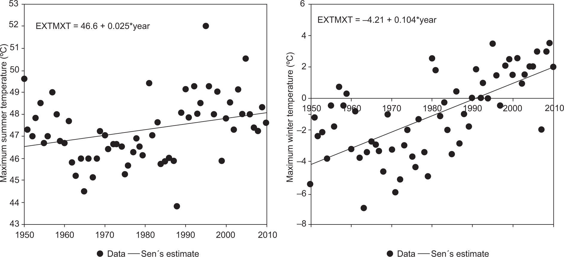
5Results5.1Temperature trendsResults of the trend analysis are summarized in Table I, and can be seen in Figure 2. In both temperature extremes, there is an increasing trend that is significant at the 95% confidence level in the case of extreme maximum temperature (EXTMXT), and at the 99% confidence level for extreme minimum temperature (EXTMNT). In particular, the extreme minimum temperature trends appear to be associated with urban growth and local land use change in the vicinity of the weather measurement site (García-Cueto et al., 2009).
Annual trends in extreme maximum temperature (EXTMXT) and extreme minimum temperature (EXTMNT) at the Mexicali weather station for the period 1950-2010. Trend analysis with non-parametric Kendall tau test (Sen’s slope estimate, standard error [SE] of the slope, and significance of the test).
Maximum and minimum temperature extreme data were drawn from annual blocks on the period 1950-2010, with a total of 61 points each. The likelihood function of the GEV for extreme maximum temperatures (EXTMXT) and extreme minimum temperatures (EXTMNT) produced the following results:
For the EXTMXT parameter, estimators (μ, σ, ξ) = (46.69, 1.39, −0.161), with standard errors of 0.19, 0.13, and 0.07, respectively. Combining the estimates and standard errors, the 95% confidence intervals (CIs) for EXTMXT are (46.31, 47.07) for μ, (1.13, 1.66) for σ, and (−0024, −0298) for ξ.
For EXTMNT, estimators (μ, σ, ξ) = (0.13, 2.53, −0.27), with standard errors of 0.36, 0.27, and 0.1, respectively. For EXTMNT, the 95% CIs are (0.49, 0.29) for μ, (2.80, 2.26) for σ, and (−0.37, −0.17) for ξ. The shape parameter (ξ) is negative in both cases of extreme temperatures; therefore, the Weibull distribution fits this data set well. Both extreme temperatures have an upper limit, so there are finite values that cannot be exceeded. The diagnostic plots used to evaluate the precision of the GEV adjusted to EXTMNT and EXTMXT are shown in Figure 3.
Probability and quantile plots show the validity of the proposed model: each set of points follows a quasi-linear behavior. As a result of the negative estimator of parameter ξ, return level curves are nonlinear. The corresponding density function appears to be consistent with the histogram data, much more so with EXTMXT than with EXTMNT, as shown in the lower right panel of Figure 3.
5.2.1Return periodsThe return periods for EXTMXT and EXTMNT are shown in the lower left panel of Figure 3, along with the 95% confidence bands estimated by the delta method. The delta method assumes that the parameter estimates are symmetric, which is not always the case for the shape parameter or large return periods.
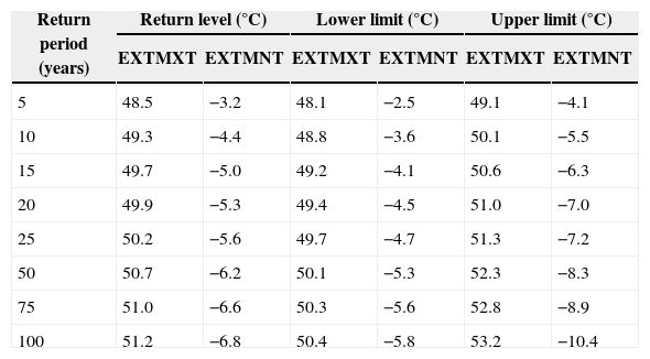
Higher precision for the CIs is generally obtained with the maximum likelihood method, so this method was applied to estimate the return periods of 5 to 100 years and the CIs. Table II shows the results using the GEV. Return levels gradually increase with larger return periods. CIs also become increasingly wider as the return periods increase.
Return levels and 95% CIs for EXTMXT and EXTMNT using the GEV distribution in Mexicali, Mexico.
| Return period (years) | Return level (°C) | Lower limit (°C) | Upper limit (°C) | |||
|---|---|---|---|---|---|---|
| EXTMXT | EXTMNT | EXTMXT | EXTMNT | EXTMXT | EXTMNT | |
| 5 | 48.5 | −3.2 | 48.1 | −2.5 | 49.1 | −4.1 |
| 10 | 49.3 | −4.4 | 48.8 | −3.6 | 50.1 | −5.5 |
| 15 | 49.7 | −5.0 | 49.2 | −4.1 | 50.6 | −6.3 |
| 20 | 49.9 | −5.3 | 49.4 | −4.5 | 51.0 | −7.0 |
| 25 | 50.2 | −5.6 | 49.7 | −4.7 | 51.3 | −7.2 |
| 50 | 50.7 | −6.2 | 50.1 | −5.3 | 52.3 | −8.3 |
| 75 | 51.0 | −6.6 | 50.3 | −5.6 | 52.8 | −8.9 |
| 100 | 51.2 | −6.8 | 50.4 | −5.8 | 53.2 | −10.4 |
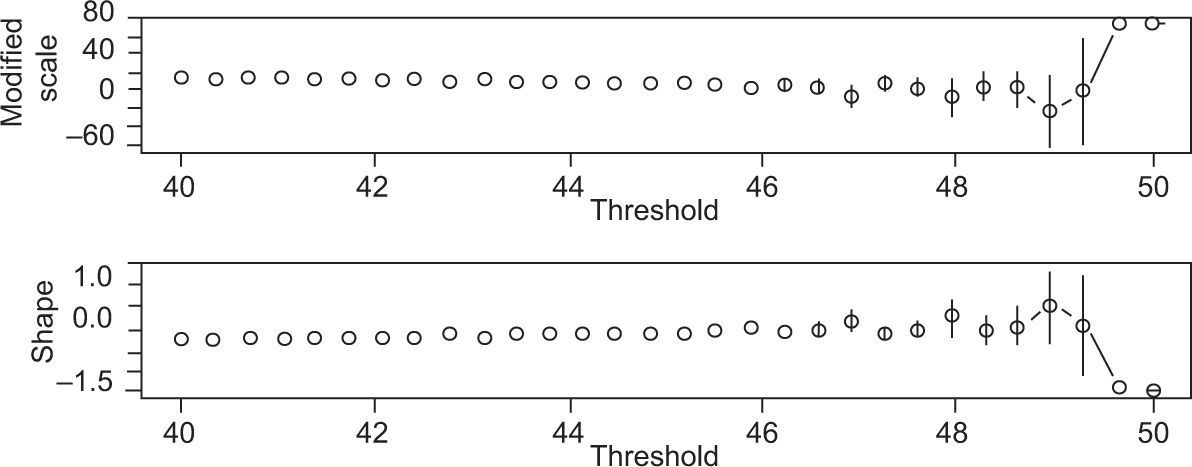
The GPD uses more information than the GEV model, which is based solely on blocks of annual values. Therefore, the GPD was adjusted to the maximum daily temperatures of Mexicali (6600 data points for the period 1950-2010). The maximum likelihood estimators of the modified scale (σ) and shape parameter (ξ) plotted versus u for the daily maximum temperatures, are shown in Figure 4. Parameter perturbations are small until the chosen threshold of 46 is reached.
The maximum likelihood estimators for the daily maximum temperatures are (σ, ξ) = (1.20, −0.14), with standard errors of 0.08 and 0.04, respectively. The 95% CIs of these parameters are (1.12, 1.28) for σ and (−0.10, −0.18) for ξ. As shown in the probability and quantile plots in Figure 5, the plotted data are quasi-linear. In accordance with negative values of ξ, the tails are finite, and the return level curves are nonlinear. The GPD model was not rejected because the likelihood ratio statistic was greater than the goodness of fit test χ2 (7.106016 > 3.84146). The p-value associated with the test is 0.00768.
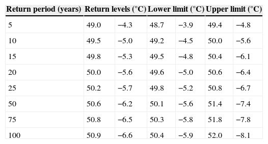
5.4Application of GPD to the minimum daily winter temperaturesFor winter minimum daily temperatures, the threshold (u) was also selected to fit the GPD. Parameter perturbations are small until the chosen threshold of −1 is reached. The estimators are (σ, ξ) = (2.18, −0.21), with standard errors of 0.14 and 0.04, respectively. The 95% CIs are (2.32, 2.04) for σ and (−0.25, −0.17) for ξ. According to the negative values of the shape parameter, the tails are finite. The GPD model was not rejected because the likelihood ratio statistic was greater than the goodness of fit test χ2 (14.96237 > 3.84146). The p-value associated with the likelihood ratio test is 0.000109. Table III shows the results of the estimated return levels and the 95% CIs for the daily maximum and minimum temperatures.
Return levels and 95% CIs obtained with the GPD for maximum and minimum daily temperatures in Mexicali, Mexico.
| Return period (years) | Return levels (°C) | Lower limit (°C) | Upper limit (°C) | |||
|---|---|---|---|---|---|---|
| 5 | 49.0 | −4.3 | 48.7 | −3.9 | 49.4 | −4.8 |
| 10 | 49.5 | −5.0 | 49.2 | −4.5 | 50.0 | −5.6 |
| 15 | 49.8 | −5.3 | 49.5 | −4.8 | 50.4 | −6.1 |
| 20 | 50.0 | −5.6 | 49.6 | −5.0 | 50.6 | −6.4 |
| 25 | 50.2 | −5.7 | 49.8 | −5.2 | 50.8 | −6.7 |
| 50 | 50.6 | −6.2 | 50.1 | −5.6 | 51.4 | −7.4 |
| 75 | 50.8 | −6.5 | 50.3 | −5.8 | 51.8 | −7.8 |
| 100 | 50.9 | −6.6 | 50.4 | −5.9 | 52.0 | −8.1 |
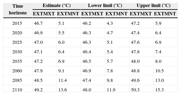
The asymptotic arguments support the use of the GEV distribution to model EXTMNT and EXTMXT, but the presence of the time trend, according to the preliminary analysis (Fig. 1) raises questions about the suitability of the conventional model that assumes a constant mean over time. The non-stationary distribution could be explained by allowing the location parameter of the GEV to depend on time. A suitable parameter for the extreme temperature in a year t, Zt, could be Zt ≈ GEV [μ(t),σ, ξ], where [μ(t) = μ0 + μ1t. The parameter µ1 corresponds to the annual rate of change in the extreme temperature series. To select the most suitable model, the likelihood ratio test was used. This test yielded a value of 38.2 for EXTMXT and 32.8 for EXTMNT, which are above the critical value of χ1,1−0.052, which is 3.84. The inclusion of a linear trend as a covariate in the GEV location parameter (μ) for EXTMNT and EXTMXT produced a significant improvement (at the 5% level). Specifically, the model obtained for the EXTMXT is μ(t) = 46.7 + 0.02567t, where t is time. By increasing the variable t, location parameter values are increasingly positive, indicating that the extreme values of maximum temperature will be more severe. For EXTMNT, the model obtained is μ(t) = −4.0 + 0.09t. The location parameter values are increasing with increasing time; therefore, the minimum temperature extremes will be less severe. Table IV shows the exceeded estimates of EXTMXT, the unsurpassed estimates of EXTMNT, and the 95% CIs (°C) obtained using the profile-likelihood method for several time horizons.
Estimated maximum (EXTMXT) and minimum (EXTMNT) temperature levels, and 95% confidence interval, using the GEV distribution and a covariable in Mexicali, Mexico.
| Time horizons | Estimate (°C) | Lower limit (°C) | Upper limit (°C) | |||
|---|---|---|---|---|---|---|
| EXTMXT | EXTMNT | EXTMXT | EXTMNT | EXTMXT | EXTMNT | |
| 2015 | 46.7 | 5.1 | 46.2 | 4.3 | 47.2 | 5.9 |
| 2020 | 46.9 | 5.5 | 46.3 | 4.7 | 47.4 | 6.4 |
| 2025 | 47.0 | 6.0 | 46.3 | 5.1 | 47.6 | 6.9 |
| 2030 | 47.1 | 6.4 | 46.4 | 5.4 | 47.8 | 7.4 |
| 2035 | 47.2 | 6.9 | 46.5 | 5.7 | 48.0 | 8.0 |
| 2060 | 47.9 | 9.1 | 46.9 | 7.8 | 48.8 | 10.5 |
| 2085 | 48.5 | 11.4 | 47.4 | 9.8 | 49.6 | 13.0 |
| 2110 | 49.2 | 13.6 | 48.0 | 11.9 | 50.3 | 15.3 |
The preliminary analysis showed a significant positive trend in both the extreme maximum temperature and the extreme minimum temperature, which is consistent with Englehart and Douglas (2005), Labajo et al., (2012), and Pavía (2008). Unlike these studies, however, the Mexicali trend in extreme minimum temperature (1.04 °C/decade) is greater than the trend in extreme maximum temperature (0.25 °C/decade). In the case of extreme minimum temperature, the marked tendency appears to be related to changes in land use in the vicinity of the weather measurement location. Materials used in urbanization (asphalt, concrete, brick, glass, etc.) have been present throughout the environment since the mid-1980s within the city and in surrounding areas. Sites that had native or agricultural soil until a few years ago are now concrete slabs. Therefore, urban development has contributed in the usual way to a tendency for higher values of minimum temperature, which is in agreement with the study by García-Cueto et al. (2009), who detected the development of an urban heat island in the city of Mexicali.
Regarding the comparative return values of extreme high temperatures, the values of the GEV and GPD are markedly similar. However, because the GPD uses more input values for modeling than the GEV (6600 data points versus 61 data points), confidence intervals are smaller in the GPD. By taking the time trend of EXTMXT into account and submitting the modeling to a non-stationary process with the GEV, the modeling is improved at a significance level of 5%. According to the probabilities estimated with the 95% CIs for different time horizons (return periods in the language of a stationary model), values are noticeably lower compared with return periods estimated with a stationary GEV and GPD; these differences range from 1.7 to 3.0 °C. It must be considered, however, that in any of the three model simulations, future extreme values are extremely high and therefore indicate increased risk.
The modeling of extreme minimum temperatures merits separate commentary. The stationary GEV and GPD models estimate increasingly negative return values for increasingly larger return periods, which clearly result in an erroneous idea of the changing process of this parameter. By including the positive trend in the location parameter of the non-stationary GEV model, as the extrapolated time horizon advances, the probability of obtaining a negative value is zero because all of the estimated values are positive; for the closest period (2015) and in the longer term (2110), it is expected (with 95% probability) that the EXTMNT does not exceed 5.1 and 13.6 °C, respectively. Therefore, it is noteworthy that under a changing climate, the proposed statistically adjusted modeling of extreme values that does not take into account observed climate trends and that is used for extrapolation will provide future scenarios far removed from the possible reality.
The foreseeable consequences of the estimated extreme maximum temperatures determined with a non-stationary GEV are unfortunately not good. Given that deaths from heat stroke due to heat waves have been reported in Mexicali in the past (García-Cueto et al., 2010), a possible scenario is that if future EXTMXT trends are not considered, coupled with other risk factors such as age, health, outdoor activity, and socioeconomic factors (like poverty and social isolation) cases of death will continue to occur and may possibly increase, essentially due to the increase in urban population and the aging of the current population; this is consistent with the findings of Furió and Meneu (2010). It is clear that measures that increase resilience might be agents of change in this scenario of foreseeable risk. Another unwanted negative impact is the increase in electricity use during the summer, as a result of increase in extreme high temperatures, to maintain indoor comfort by using air-conditioning equipment for longer periods of time.
As for the EXTMNT, because higher values are estimated, which corresponds to less severe winters than those currently observed, it is anticipated that expenditures for electric heating will decrease noticeably; additionally, the urban ecosystem, particularly the flora and fauna, will experience fewer effects caused by low temperatures. Even vulnerable groups such as children and the elderly may have fewer respiratory problems.
Based on the results obtained with the theory of extreme values, by modeling the non-stationary GEV, i.e., incorporating climate change by way of the trends of both extreme temperatures, it is statistically reasonable to expect an increasingly warmer urban atmosphere, both in future summers and winters. However, other approaches to study changing extreme event conditions, such as the applications of regional climate models (whether dynamic or statistical) that include the release of greenhouse gases into the atmosphere, need to be included in future research.
7ConclusionsAn increasing, significant annual trend was observed in the EXTMNT and EXTMXT; both series are non-stationary. A more pronounced warming was observed in the EXTMNT that can be associated with urbanization. The GEV distribution and GPD were adequately fitted to both temperature extremes, but extrapolation with the return periods has some shortcomings. The inclusion of the time trend as a covariable in the location parameter produced a significant improvement (at 95%) in the GEV, especially for the EXTMNT; therefore, individuals assessing impacts in several areas should use the values shown in Table IV. It can be observed that by the end of twenty-first century the extreme maximum temperature could be 2 to 3° C higher than current, and the winter could be less severe, as the extreme minimum temperature, according to the probabilistic model, suggests increases of 7 to 9 °C with respect to the base period (1950-2010). Although the GPD uses daily values, it fails to integrate a temporal trend in modeling, which makes its application to climate change issues questionable.


