La densidad de potencia, los perfiles verticales de velocidad y otras características del viento se establecieron por medio de una torre meteorológica de 51m localizada muy cerca de la línea costera en el noroeste de la península de Yucatán, ubicada en el golfo de México. Se llevó a cabo un estudio comparativo de la densidad de potencia del viento utilizando información obtenida de septiembre de 2010 a septiembre de 2011. Se encontró que la función de densidad de probabilidad para la velocidad del viento es bimodal a causa de las brisas que soplan de mar a tierra, característica menos evidente a medida que aumenta la distancia vertical al suelo. La diferencia entre estos dos regímenes de viento se utilizó para ajustar la curva de Weibull-Weibull usando un criterio de mínimos cuadrados lineales en los parámetros. Adicionalmente, las simulaciones numéricas de un modelo de mesoescala concuerdan con las mediciones por arriba de z=50m (z es la distancia vertical al suelo). Esto sugiere que algunas simulaciones de mesoescala pueden servir como herramienta preliminar para valorar la energía del viento en zonas costeras con extensas áreas bajas.
Wind power density, vertical velocity profiles, and other wind characteristics were established using a 51 m meteorological mast located very close to the shoreline on the northwest of the Yucatan peninsula in the Gulf of Mexico. A comparative study of the wind power density was carried out using information obtained between September 2010 and September 2011. The wind speed probability density function was found to be bimodal due to sea-land breezes, a characteristic that becomes less evident as the vertical distance to the ground increases. The distinction between these two wind regimes was used to fit the Weibull-Weibull curve using a linear least-squares criterion in the parameters. In addition, numerical simulations from a mesoscale model are in close agreement with measurements above z=50m (z is the vertical distance to the ground). This result suggests that some mesoscale simulations may serve as a preliminary wind energy assessment tool in coastal zones with extended low-lying areas.
Wind power technology has been evolving through the history of mankind for at least 3000 years (Sathyajith, 2006). During the last decades, it has experienced unprecedented growth rates due to the transition to sustainable development, triggered in the 1970s by several factors: the oil crisis of 1973 and 1979, the discovery of the ozone layer depletion caused by chlorofluorocarbon aerosols in the upper atmosphere (Molina and Rowland, 1974) and the global warming due to the greenhouse effect related to some gaseous emissions like C02 or CH4 to the atmosphere (Broecker, 1975). This tendency has been reinforced by the development of a gradual ecological consciousness and important international actions such as the Kyoto Protocol in 1997 and 2005. Between 2004 and 2009 the worldwide cumulative wind power capacity grew in average 27% (REN21,2010).
The efforts to transform the energy and industrial sectors to use renewable energy have been successful in some countries like the United States of America. China, Germany and Spain. In developing countries an important growth is also observed, notwithstanding the economical difficulties. Mexico is not an exception to this trend, and in 2005 an 83 MW wind farm was built in La Venta, on the Tehuantepec Isthmus in the state of Oaxaca, Mexico. A total installed power of more than 580MW is projected by the end of 2012 in that same region (SENER-CFE, 2009).
Considering other regions, the wind potential in Mexico is not particularly abundant with the exception of some particular locations known to have strong winds all year round, according to data collected by standard meteorological stations throughout the country. There are few studies that estimate the power density (power/unit of area), whose results are based on experimental facilities specialized on wind energy assessment (Saldaña and Miranda, 2005). In the case of Sisal, Yucatan, there is a previous work (Saldaña and Miranda, 2009), where the power density was established using a mast equipped with cup anemometers at z=20 and 40m. Wind data was collected during the period comprised between January 2005 and September 2007. Information about the wind roses, Weibull curves and their corresponding parameters, as well as wind speed averages are available for direct comparison. The power density was estimated to be D=222 and 298 W/m2 at 20 and 40 m, respectively, and a projection for 80 m was also obtained using a power law fit for the vertical wind speed profile. To our best knowledge, this is the only previous study in Sisal; however, there are other previous investigations in Yucatan (Soler-Bientz et al., 2011) where the offshore potential and temperature profiles were studied, as well as the wind shear patterns on an inland site near Merida, 50 km away from Sisal (Soler-Bientz et al., 2009).
All these contributions mention the strong influence of the coastline on the weather and wind patterns, which result from strong temperature and humidity gradients, as well as the sudden roughness step found at the shoreline. Some aspects of these complex interactions, such as the correct scaling that describe atmospheric stability near internal boundary layers still present an important challenge for scientists and engineers, who require a precise assessment of the wind resource.
The evaluation of the wind power potential can be achieved using rather standardized techniques (Rohatgui and Nelson, 1994), which work well in a variety of situations and terrain characteristics. The usual viewpoint is to evaluate the power density (in W/m2) by means of the wind speed probability distribution function (PDF). If the data is collected for a long period of time (larger than one year) this PDF can be approximated to a theoretical curve, like the Rayleigh or Weibull PDF (Justus et al., 1978). However, this is not feasible for some complex terrains, as was documented by Romero et al (2003) and Jaramillo and Borja (2004) for La Ventosa, located in the state of Oaxaca, Mexico. It was observed that the PDF is bimodal, with high wind speeds coming from the north-northwest as a result of wind channeling from the Gulf of Mexico to the Pacific Ocean through the Isthmus of Tehuantepec, mainly driven by pressure differences between the two basins. Winds from other directions, as well as local effects (such as the ocean breeze) contribute to the second peak of the PDF (at lower wind speed).
Other types of PDF can be fit to bimodal data, such as the so-called MEP (minimum entropy principle) type distribution described by Li and Li (2005) and used in a comparative study (Chang, 2010) where different PDF’s were tested with experimental data. The Weibull-Weibull (WW) curve, as well as the MEP-type distributions proved to be well suited for some wind regimes found over complex terrain. The WW curve was chosen for the characterization of wind speed PDF in this study for two reasons: as already stated, it is well adapted for the description of bimodal wind regimes, and for simplicity, as will be shown in section 3.
2Objectives and limitationsThe present study was motivated by a collaborative effort between different research and industrial partners (see the Acknowledgments section) in order to assess the wind power potential in the northwest of the Yucatan peninsula, in the Gulf of Mexico. The objective of this study is to characterize wind resources using statistical tools such as the probability distribution function of wind velocity. Some diurnal, monthly and seasonal averaging of other variables (such as wind direction) are also reported and used to improve the power density estimation. A methodology for fitting the wind speed PDF based on the diurnal breeze regime is proposed and tested with experimental data. Additionally, a comparison between the experimental results and numerical mesoscale simulations is presented. These simulations were carried out at the Centro de Ciencias de la Atmósfera (CCA) of the Universidad Nacional Autónoma de Mexico (UNAM), located in Mexico City. This report will not cover turbulence characterization, which will be reported elsewhere in the future. However, for completeness, and because the calculation of some turbulent quantities require special considerations, such as the use of the eddy correlation technique, the most important steps in the pre-processing stage are covered in section 5.
The present document is organized as follows: firstly, the WW PDF is introduced in section 3 in order to justify the proposed methodology. Next, the experimental setup will be treated in section 4, where the location, instrumentation and data acquisition are described. The pre-processing of the experimental data is discussed in section 5, and the results are presented in section 6 in terms of wind direction, wind speed PDF, and power density; a comparison with results from the mesoscale simulations and the literature are also shown. Finally, in section 7 the results are summarized, along with some comments and perspectives.
3Theoretical backgroundThe Weibull distribution is a two-parameter PDF, given by
where k (dimensionless) and A (m/s) are the shape and scale parameters, respectively. The mean and standard deviation of the respective PDF are given by Hennessy (1977):
and
where U is the mean wind speed and Γ is the gamma function, defined as:
The WW curve is defined simply as a weighted sum of two Weibull curves (e.g., Jaramillo and Borja, 2004, and references therein):
where subscripts indicate the existence of two PDF’s, and the weighting factors p and (p−1) can be interpreted as the probability distribution of two mutually exclusive events. The expected power density D can be related to the PDF as follows:
where P(U) is the power of the wind moving at an average speed U through an area A, and ρ is the corresponding air density. For the case of a WW distribution, the power density is (Jaramillo and Borja, 2004):
Let us remark that in coastal zones it is common to find a daily pattern of sea-land breezes; due to the large difference in surface temperature and roughness between sea and land, there is a distinctive regime that characterizes the wind coming from each environment. If the direction of the wind is known, then it could be stated that the weighting factor p is also given (e.g., as the probability that a given set of data comes from the sea). If both regimes are separated using this distinction, and the parameters are calculated from a unimodal Weibull PDF and then combined through the weighting factor p given by the aforementioned probability, the WW bimodal curves could easily be fitted using standard parameter estimation methods. Moreover, a unimodal Weibull curve can be fitted using a linear least squares criterion in the parameters to minimize the error (Tuller and Brett, 1983). The parameter estimation procedure can be carried out without the need of nonlinear methods (which are dependent on a suitable first guess, among other problems). In section 6 it will be shown that this methodology is pertinent at least for the particular case of Sisal. We believe that it also applies to any coastal zone with a well-defined regime of sea-land breezes, excluding complex terrains with prominent hills or cliffs, where re-circulations and other phenomena may require special treatment.
4Experimental setupThe experiment is located at 90° 02’ 48” W, 21° 09’ 53” N, at approximately 120 m from the shoreline in the coast of Yucatan, as shown in Figure 1. The insert at the lower left is an aerial photograph of Sisal, which is a small fishing town whose port used to be of great importance up to the late nineteenth century, when the more modern port of Progreso was built to the east, only 25 minutes from Mérida, capital city of the Yucatan state (the name Sisal comes from a plant of the Agave genus whose fibers are used to make twine and rope).
A meteorological mast is located at the campus of the Universidad Nacional Autónoma de México in Sisal, to the north of an artificial shelter harbor (see the arrow near the upper left of the insert). To the south there is a marshland (flooded during the rainy season), followed by a dense mangrove forest. Farther to the south there is a subtropical dry broadleaf forest that transitions gradually into an agricultural patchy terrain until the city of Hunucma, 20 km away.
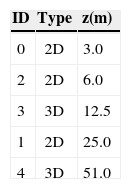
The meteorological mast is 51 m high, and is equipped with five ultrasonic anemometers: three of the 2D 4.382xx family, and two of the 3D 4.3830xx family (Adolf Thies GmbH and Co.). These instruments can report two or three wind velocity components and a meteorological variable usually known as sonic temperature, which is a good approximation to the virtual potential temperature (Kaimal and Gaynor, 1991) even under humid conditions near the sea level provided that only the fluctuations are involved in the calculations. The acquisition frequency for the sonic anemometers is 10 Hz, which allows for the analysis of several micrometeorological parameters such as turbulent intensity, kinematic heat and momentum turbulent transport, Monin-Obukhov length and friction velocity. However, most of the results in this report do not require high frequency measurements. The anemometers were located at 3,6, 12.5,25 and 51 m above the ground level, respectively, distributed as shown in Table I.
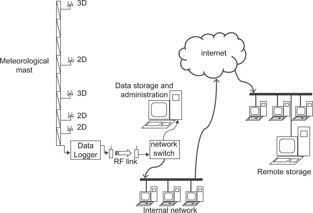
At the base of the tower a Data-Logger (DL) NDL485 (Wilmers Messtechnik GmbH), interrogates the anemometers and stores the readings in its internal memory, capable of retaining about eight hours of high frequency data stored in ASCII file format, each file containing one hour of experimental data. The DL is connected to the network via a radio-frequency (RF) link (using radios and two directional Yagui antennas), which in turn is connected to a network switch, as shown in Figure 2. This switch allows for the communication with a file server, which retrieves the information from the DL every two hours. Each file contained an hour of high frequency data (about 3 MB of data), which could overload the wireless communication link if the files were immediately downloaded to the server. The two-hour data retrieval period proved to be robust enough to allow for the DL to perform its acquisition and communication tasks safely. Additionally, a remote server in Mexico City performs the same data retrieving routine in order to have a backup copy in case of failure of the main computer (see “Remote storage” in Fig. 2). This setup permits the correct data retrieving in case that the internal network is temporarily down, and allows for real-time access to the DL. Two solar panels and a rechargeable (deep cycle) battery provide energy to the sonic anemometers, the DL, and the RF radio transmitter. The data storage and administration tasks comprise storing the raw data files and the maintenance of an online OpenSource database where average data is stored for collaboration with other colleagues and institutions. This database also contains a table with other meteorological variables coming from a meteorological station located at the base of the tower (z=1.5m).
5Data processingFirstly, the data was treated for quality control purposes. A set of operations to select and treat the signals before averaging (or calculating turbulent quantities) is discussed in this section. One important parameter to take into account is the averaging period, which ranges from 30 min to 1 h in micrometeoro-logical studies. An Ogive test (Oncley et al., 1990; Foken and Wichura, 1996) was carried out in order to evaluate this time scale, with a resulting period of 25 to 30 min for the averaging time used to obtain first and second moments of the relevant variables. The raw data was subjected to different validations:
- a.
All the files containing incomplete or clearly erroneous data were discarded. After a visual inspection many files were also discarded. Unfortunately, it was impossible to visually inspect all files (more than 6000).
- b.
Files with missing data were also discarded (we chose an arbitrary threshold of one second). Smaller gaps were filled using an interpolation procedure based on a filtered version of the signal. There were many small gaps with periods smaller or equal than 0.2 s (26%), but the total number of gaps between 0.3 s and 1 s was only 0.5%.
- c.
A stationarity test (Foken and Wichura, 1996) was implemented to qualify the time variation of statistics at different time intervals, with a threshold of 30% of tolerance for the variances.
- d.
A three rotation scheme of the wind vector was carried out (Kaimal and Finnigan, 1993), such as to obtain w¯=0, v¯=0 and vw¯=0.
The wind velocity data was later processed in order to obtain averages and moments of the microme-teorological variables at hand, and saved in order to perform further analyses. The results that correspond to wind power density are presented in the following section. Note that in this particular experiment raw data is also recorded digitally, so all pre- and post-processing can be done again in the future, allowing for the correction and trial/proposal/implementation of new processing techniques and analyses.
6ResultsThe results are divided in two subsections. The first one presents some qualitative description of the average weather conditions in Sisal, before reporting the average wind direction with respect to different periods of time. This information is important in order to understand the cycles that characterize the site and its wind energy potential. The second subsection is devoted to the PDF parameter estimation and the calculation of the wind power density at different heights from the ground, which was compared with a meso-scale numerical model. These simulations were done with the Weather Research and Forecasting (WRF) model, which is a mesoscale numerical weather prediction model that comprises several solvers and applications, based on a numerical Eulerian solver for the fully compressible non-hydrostatic equations, cast in flux-conservative form, using a mass (hydrostatic pressure) vertical coordinate (Skamarock et al., 2005). This code is freely available from the WRF model webpage (http://www.wrf-model.org/index.php). The simulated data comes from a project related to weather forecasting (and other applications, such as pollution dispersion) that covers the whole Mexican territory. The boundary conditions are taken from the Global Forecast System, and are run locally with a spatial resolution of 0.187º in the Yucatan peninsula.
6.1Wind directionThe weather of Sisal, Yucatan is warm and humid, with average temperatures that go from 22 °C before sunrise to 29 °C at midday hours. Average humidity is usually over 85% and falls at noon to values near 75%. Atmospheric pressure varies from year to year, with a cycle that shows a couple of troughs at 3:00 am and 6:00 pm (local time) ranging from 101 100 to 101 600 Pa. Wind velocities are large compared to nearby locations in the Yucatan peninsula, and can be as much as 50% stronger than the wind in Celestuán, 50 km away to the southeast. Dominant winds come from the northeast and southeast, and there exists a pattern of repetitive winter events (cold fronts known locally as Nortes) coming from the north with violent winds, rain and significant temperature drop. There is a rainy season during the summer, where the average wind speed falls considerably, as will be shown shortly. The more energetic winds come from tropical storms and hurricanes that usually pass by towards the coast of the states of Veracruz and Tamaulipas, or to the north towards Texas or Louisiana in the USA.
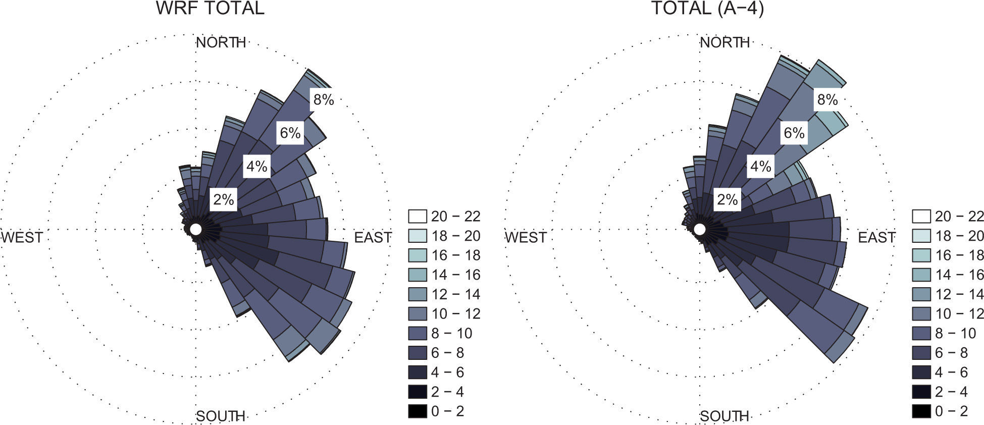
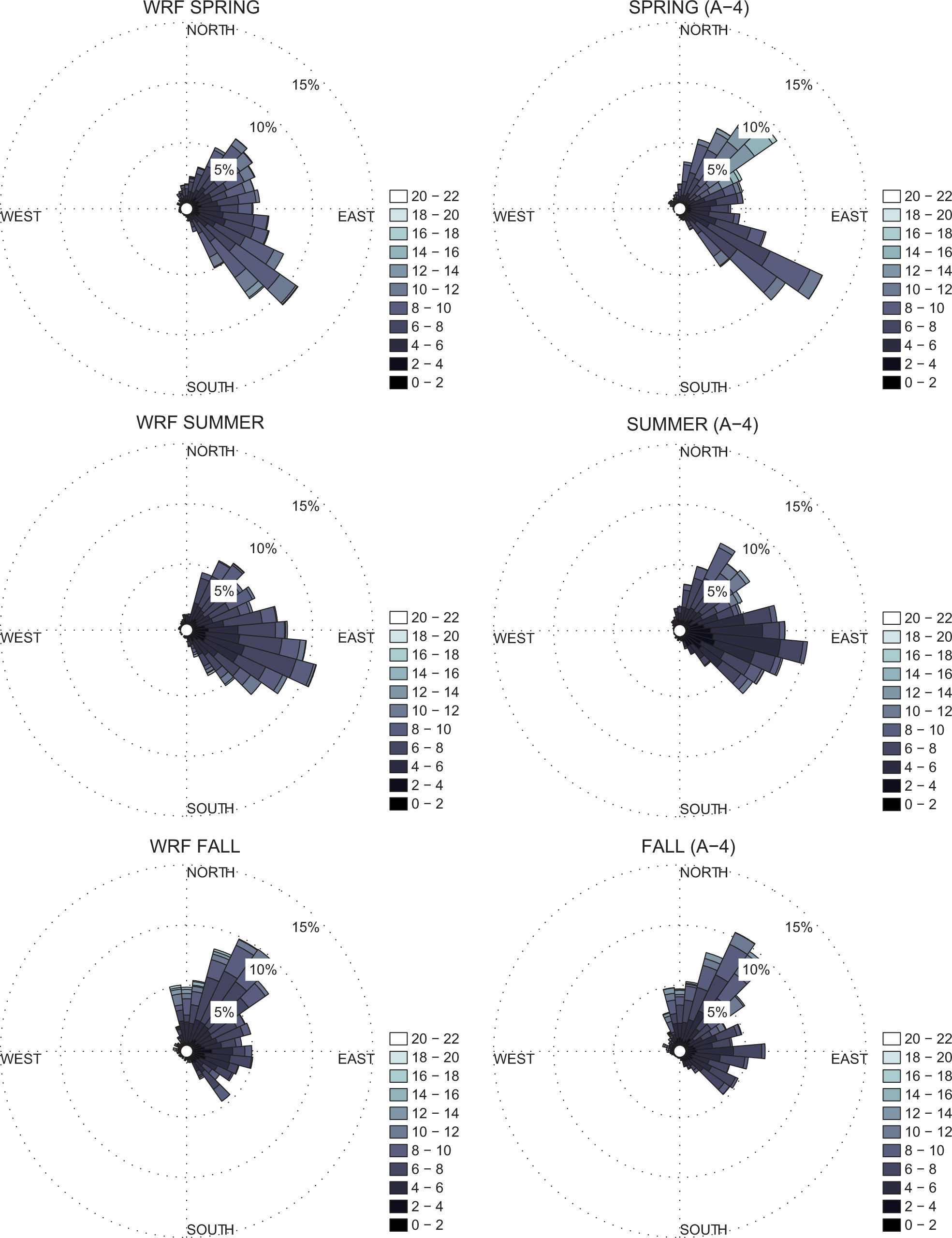
The wind speed and direction are presented in Figure 3 in the form of wind roses: to the right, the experimental data at 50 m is presented. The sub-figure to the left comes from averaging the WRF simulation data. Both results are very similar, but one can observe that some differences arise in terms of wind speed. The figure also shows that the more energetic winds come from the northeast, while the most frequent direction is the southeast. The same data, averaged seasonally, is presented in Figure. 4; again, the simulations can reproduce the behavior of the wind correctly. Note that the WRF wind rose for the winter is different from that of the mast, particularly for the southeast, where the mast presents a large frequency peak. Winds coming from that precise direction pass over the marshland and are then channeled to the mast through a terrain where there are very few buildings, so it is reasonable to assume that these differences in the wind roses are due to the complex terrain configuration (not taken into account by the WRF model). Comparisons between the anemometer at z=12.5m can also be made, since the WRF model gives the velocity at z=10m, and although there are similarities, sharp differences exist, as will be evident from the PDFs shown in Figure 6.
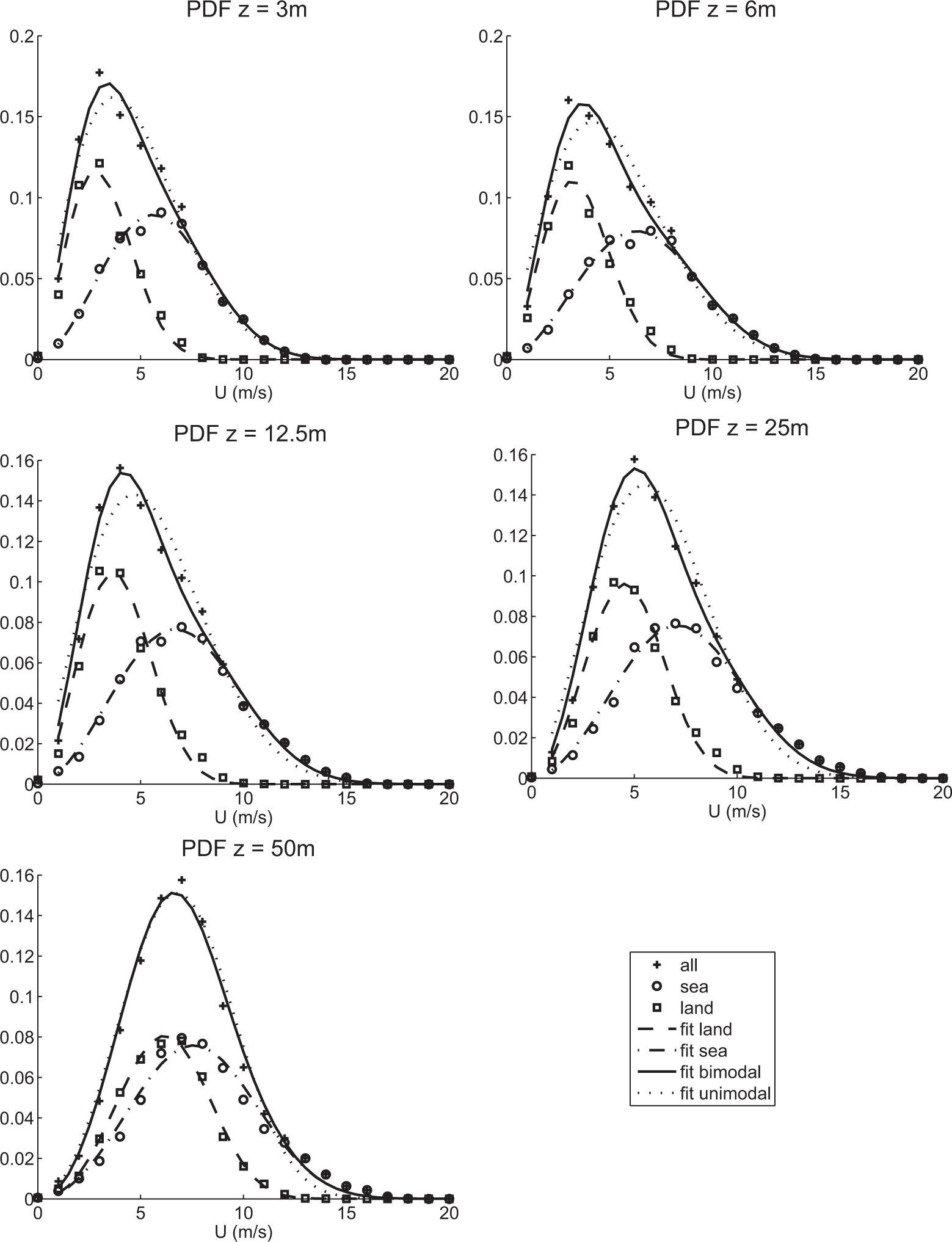
As already outlined in previous sections, the method to fit the WW distributions to the data is as follows: first, we estimate the probability p of getting winds coming from the sea as:
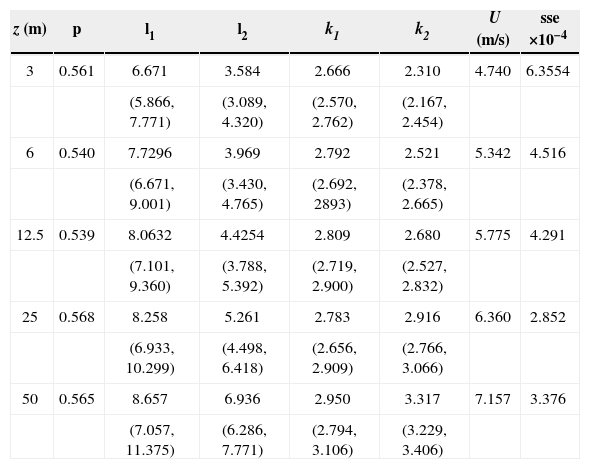
where Nsea is the number of events in which the average wind direction came from the sea, and Ntotal is the total count of events (about 14 000 30-min events). The next step is to separate all the experimental points coming from the sea, and fitting a Weibull curve (with a least squares criterion) to obtain its corresponding k1 and λ1 Then, the same process is carried over with the data coming from land, in order to get k2 and λ2. The results are presented in Figure 5, where the PDF for winds coming from the sea (circles), land (squares), and all directions (crosses) is presented, for five different heights above the ground. The bimodal character of the curve is clear for low heights (z=3 and 6m), where a “hump” coming from the larger wind velocities from offshore is apparent. As the height above the ground increases, this feature is less evident, as can be seen from z=25 and 50m. The bimodal fit is in all cases better than the unimodal one; for example, at z=50m the WW fit gives a sum of squared errors sse=0.3376 × 10⁻³, while the corresponding error for a W fit is sse=0.7816 × 10⁻³. The parameters and their corresponding confidence intervals are listed in Table II.
Weibull-Weibull PDF parameters and corresponding standard errors for different heights above the ground (95% confidence intervals shown in parentheses).
| z (m) | p | l1 | l2 | k1 | k2 | U (m/s) | sse ×10−4 |
|---|---|---|---|---|---|---|---|
| 3 | 0.561 | 6.671 | 3.584 | 2.666 | 2.310 | 4.740 | 6.3554 |
| (5.866, 7.771) | (3.089, 4.320) | (2.570, 2.762) | (2.167, 2.454) | ||||
| 6 | 0.540 | 7.7296 | 3.969 | 2.792 | 2.521 | 5.342 | 4.516 |
| (6.671, 9.001) | (3.430, 4.765) | (2.692, 2893) | (2.378, 2.665) | ||||
| 12.5 | 0.539 | 8.0632 | 4.4254 | 2.809 | 2.680 | 5.775 | 4.291 |
| (7.101, 9.360) | (3.788, 5.392) | (2.719, 2.900) | (2.527, 2.832) | ||||
| 25 | 0.568 | 8.258 | 5.261 | 2.783 | 2.916 | 6.360 | 2.852 |
| (6.933, 10.299) | (4.498, 6.418) | (2.656, 2.909) | (2.766, 3.066) | ||||
| 50 | 0.565 | 8.657 | 6.936 | 2.950 | 3.317 | 7.157 | 3.376 |
| (7.057, 11.375) | (6.286, 7.771) | (2.794, 3.106) | (3.229, 3.406) |
When compared with the PDF from the WRF me-soscale model, the experimental curves differ considerably for low heights, as shown in Figure 6, where the curves corresponding to z=10m obtained numerically (crosses) and the one corresponding to the mast at z=12.5m are presented. On the other hand, above z=50m the model obtained very reasonable results, shown in Figure 6b. The reason for this discrepancy at low heights is the parameterization of the surface layer in the numerical model; the conditions of both offshore and onshore winds are perturbed by the presence of internal boundary layers. Above the influence of these perturbed profiles the numerical prediction does a much better forecast. The complexity of the terrain, as well as land-sea interface play an important role in wind characterization. These effects are not taken into account in mesoscale models because of the coarseness of the grid, and could be parameterized using the state of the art of internal boundary layers (Savelyev and Taylor, 2005); however, the introduction of such effects is very likely to require a mesh refinement (e.g., along the coastline), which in turn implies necessarily some computational cost. The effects of topography at the micrometeorological scale can be assessed by taking the mesoscale simulation as the input for a microscale simulation; this is a very active field of research (Churchfield et al., 2010; Jonkman, 2013; Serrano et al., 2014) in view of the transition to clean energy production, which will be implemented during the first half of this century.
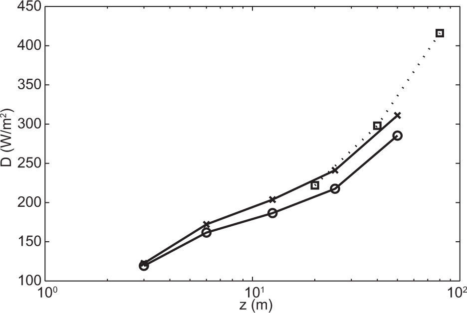
Power densities (W/m2) as a function of height z are shown in Figure 7, where crosses represent the power density Db obtained with a WW PDF (this study), circles represent the unimodal power density Du, and the results of Saldaña and Miranda (2009). which are unimodal, are shown as squares. There is good agreement in terms of the power densities Db (this study) and DuS (Saldaña and Miranda, 2009). The corresponding unimodal parameters k and λ are shown in Figure 8, for completeness. These parameters are similar in both studies; however, there is a significant difference between the unimodal power densities DuS and Du. The results of Saldaña and Miranda (2009) were obtained during a 3-year observation period, while our data covered only one year; our bimodal estimations of the power density are very similar to those obtained by these authors, so it is more likely that our bimodal estimations are more precise than the corresponding 1-year unimodal versions. The point corresponding to z=80m in Figure 8 is a projection calculated in Saldaña and Miranda (2009) by means of a power law; however, this kind of prediction is hard to justify in view of the presence of boundary layers and the additional complexity that arises when working above the surface layer (Soler-Bientz et al., 2009). The possibility of extending the wind profiles above the surface layer has been also explored by Kelly, and Gryning (2010), who considered an adaptation of the well-known Obukhov theory from the probabilistic point of view for the surface layer, in order to obtain long-term wind profiles based on common surface layer parameters and the effect of the atmospheric boundary layer depth. Gryning et al. (2007) considered in a more direct way the problem of extending the wind velocity profile taking into account the pertinent length scales that control the velocity in a three-layered model for the entire atmospheric boundary layer height. These studies require, in general, the knowledge of parameters such as the Obukhov length L, friction velocity u*, boundary layer height z1, etc. This task was left out of the scope of the present paper.
Comparison between the power density obtained by Saldaña et al. (2009) and the present study. ×: Db present study; o: Du present study; □: DuSSaldaña et al. (2009).
Comparison between the power density parameters. Symbols: ×: k present study; ◊ : kSaldaña et al. (2009); o: λ present study; □: λ Saldaña et al. (2009).
The wind power density at Sisal, located at the northwest of the Yucatan peninsula in the Gulf of Mexico was estimated from a meteorological mast experiment. It was observed that the experimental PDF was bimodal, due to the presence of two distinct regimes: winds from land and from the sea, the latter showing larger wind velocities, while the former are more frequent. For small heights above the ground, bimodality was evident, and as the top of the mast is reached at z=50m, PDFs look more unimodal; however the quadratic error is still smaller for the bimodal fit. The parameters were estimated using linear least squares of each regime separately, since the probability p of having winds from the sea is known from the measurements. This methodology has the advantage of being linear in the parameters so there is no need of nonlinear search methods or an initial guess. It can also be carried out using simple programs such as computer worksheets. The results were compared with the only previous work in the literature for Sisal, as well as with numerical mesoscale simulations carried out at the CCA in Mexico City with the WRF model. For heights above 50 m it was shown that the mesoscale simulations are remarkably accurate, so the use of such tools as preliminary resource assessment looks promising. Further research is being done to validate a reliable methodology.
The authors respectfully acknowledge the support of Conacyt, CFE and the Government of the State of Yucatan through projects FONSEC-CFE 89073 and FOMIX 106400, as well as the help of the staff of the Instituto de Ingeniería and the Centro de Ciencias de la Atmósfera (UNAM), the T. A. Octavio Gomez R., and the students Elsa Hernandez J. and Sareti Cardos P. We are also thankful of the Instituto de Investigaciones Eléctricas and Dr. Ubaldo Miranda M. for their support providing space in their meteorological tower.


