Retrospective health impact assessment for ozone pollution in Mexico City from 1991 to 2011

Resumen

La contaminación atmosférica es el principal problema ambiental en la ciudad de México, donde el ozono es uno de los contaminantes que mayor daño causa a la salud humana. En este trabajo se presenta un análisis retrospectivo del impacto sanitario de las políticas regulatorias de contaminación por ozono desde 1991 hasta 2011 en la zona metropolitana del Valle de México. El estudio se divide en grupos etarios, ya que éstos presentan diferencias respecto a la vulnerabilidad. Dado que las personas se mueven de un lugar a otro durante el día, lo cual puede afectar su exposición potencial a los contaminantes, se consideran distribuciones espaciales de población variables durante el día. Los datos de ozono consisten en registros tomados con frecuencia horaria desde el 1 de enero de 1991 hasta el 31 de diciembre de 2011, en 22 estaciones de la red de monitoreo atmosférico de la ciudad de México. Sin embargo, considerar estos registros es insuficiente; también es necesario interpolar los valores para localizaciones no medidas. El análisis objetivo de Cressman fue el método utilizado para llevar a cabo la interpolación de concentraciones de ozono hacia retículas de resolución conveniente. Se demuestra que los diferentes grupos etarios presentan diferentes patrones espaciales de exposición, y que las personas en edad laboral (de 18 a 64 años) son las más beneficiadas. También se confirma la hipótesis de que en general las personas se mueven hacia regiones menos contaminadas durante el día.

Abstract

Air pollution is the main environmental issue in Mexico City, where ozone is one of the most damaging pollutants for human health. In this work we present a retrospective health impact assessment (HIA) study split up by age groups for evaluating the benefits of ozone regulatory strategies from 1991 to 2011 in Mexico City. Since people move from one place to another during the day, which may affect their potential exposure to pollutants, we consider time-dependant spatial population distributions during the day. Ozone data is made up of observations taken with hourly frequency from January 1, 1991 to December 31, 2011, at approximately 22 stations of the monitoring network of Mexico City. Interpolated values for unknown locations are also taken into account in the HIA. The Cressman objective analysis method is applied for interpolating the observed ozone concentrations from monitoring stations to grids of convenient resolution. We demonstrate that different age groups present different spatial patterns of exposure, being the working-age people (between 18 and 64 years) the most benefited. We also confirm the hypothesis that, in general, people move to less polluted regions during the day.

1

Introduction

Over the last two decades, several public health studies have confirmed the statistically significant associations between outdoor concentrations of tropospheric ozone and a wide range of adverse outcomes (Ostro et al., 2006), including premature mortality, hospital admissions for respiratory disease, urgent care visits, asthma attacks and restrictions in activity.

In Mexico City, atmospheric pollution is the main environmental issue. According to the 2010 air quality report for Mexico City, published by the Sistema de Monitoreo Atmosférico (Air Quality Monitoring System) (SIMAT, 2010), air quality exhibits an important improvement for almost all the included pollutants, which is attributed to the application of different environmental prevention programs during the last 20 years. Nevertheless, in 2010 ozone and particulate matter concentrations exceeded the values established by the Mexican Official Standard in more than 40 and 28% of the days, respectively.

A research that evaluates potential and retrospective costs of pollution (or benefits of regulation strategies) is generally referred to as a health impact assessment (HIA) (Ostro et al., 2006). In this work, a retrospective HIA is presented in order to evaluate the benefits of tropospheric ozone regulatory strategies from 1991 to 2011 in Mexico City. The analysis is split up into four population groups given by age: [0, 5], [5, 18], [18, 64], (64, ∞).

The main contribution of this study is acknowledging population mobility during the day, which affects their potential exposure to pollution. Therefore, considering a dynamical spatial population distribution that changes during the day instead of a static spatial population distribution given by home locations (i.e., assuming that people stay at home during the whole day) is a more realistic approach.

Interpolated values for unknown locations are also regarded in the HIA, in addition to records of ozone concentrations at monitoring stations. The Cressman objective analysis method is applied to interpolate the observed ozone concentrations from monitoring stations to grids of convenient resolution.

2

HIA components

An HIA for ozone pollution reduction involves four elements (Ostro et al., 2006):

• 1.

  Estimation of changes in ozone concentration due to control strategies.

• 2.

  Estimation of the number of people exposed to the changes in ozone concentration.

• 3.

  Baseline incidence rate (BIR) of the adverse health outcomes associated with ozone pollution (i.e., number of health-related events per year per capita).

• 4.

  Concentration-response (CR) functions that link changes in ozone concentration with changes in the incidence of adverse health effects. These functions come from epidemiological studies and are expressed in terms of percentage of change in a given health outcome attributable to a unit change in ozone concentration.

The product of these four elements is considered as the expected number of avoided adverse health outcomes related to a control strategy. In order to generate estimates for the economic benefits, an economic valuation may be assigned to the health outcomes. Points 1 and 2 are explained in detail in the next two sections.

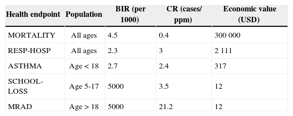
In this study, we focus on the following health outcomes:

Health endpoint	Abbreviation
Premature mortality	MORTALITY
Hospital admissions for respiratory diseases	RESP-HOSP
Emergency room visits due to asthma attacks	ASTHMA
School loss days	SCHOOL-LOSS
Minor restricted-activity days	MRAD

The values considered in this work for the HIA parameters and the affected population group (determined by age) are presented in Table I. There are different approaches for the estimation of such parameters in the literature. We follow those that have been successfully used in INE (2006), Stevens (2008), Jazcilevich et al. (2011) and Huerta-Roldán (2013), which are good enough for the simulation purposes of this study. A discussion about the accuracy and efficiency of those estimation approaches is beyond the scope of this paper.

Table I.

HIA parameters.

Health endpoint	Population	BIR (per 1000)	CR (cases/ ppm)	Economic value (USD)
MORTALITY	All ages	4.5	0.4	300 000
RESP-HOSP	All ages	2.3	3	2 111
ASTHMA	Age < 18	2.7	2.4	317
SCHOOL-LOSS	Age 5-17	5000	3.5	12
MRAD	Age > 18	5000	21.2	12

Economic valuations of health income endpoints provide a general sense of the magnitude of the societal benefits. In the literature two main economic valuation approaches are found: willingness to pay (WTP) and cost of illness (COI) (Stevens, 2008). In this context, the WTP refers to the maximum amount of money a person would be willing to pay in order to avoid an adverse health outcome, while the COI includes the cost of medical treatment, drugs and productivity loss. Available studies suggest that the WTP may be more than twice the COI, because the latter does not take into account the suffering associated with illness (Ostro et al., 2006).

The economic value of premature mortality is considered as the mean value of statistical life (VSL). There is no concept for the value of a specific human life in econometrics. However, in certain circumstances, it is desirable to have a valuation of the cost of death prevention. In order to estimate the VSL, the risks that people would be willing to take and the amount they should be paid for those risks may be considered. Another method to estimate the VSL is asking people how much they would be willing to pay for a reduction in the likelihood of dying.

3

Ozone concentration estimations

Generally, statistical analysis for air quality considers pollutant concentration records from monitoring stations. The SIMAT is responsible for watching and evaluating air quality in the region, taking into account data obtained in monitoring stations. Stations report pollutant concentrations with hourly frequency. In order to study the potential risk that population has been exposed to, additionally to stations records it is also necessary to consider pollutant concentrations for other locations, e.g. on a regular grid with the required resolution. Usually it is not possible to record pollutant concentrations at such locations, thus it is necessary to estimate them. One solution is to interpolate ozone concentrations from monitoring stations records to a regular grid. The interpolated values may be crossed with spatial population distribution data in order to evaluate the population potential exposure to pollutants.

In this work, the Cressman objective analysis method was applied for such interpolation, considering ozone concentration records taken with hourly frequency from January 1, 1991 to December 31, 2011, at approximately 22 stations of the SIMAT (2012). The three quartiles of ozone concentration by month are plotted in Figure 1, where a slow decay and certain yearly periodic pattern can be noted.

Fig. 1.

Ozone by month.

A spatial interpolation was carried out for each one of the 184 080 hours encompassed. The Cressman method is summarized below.

3.1

Cressman objective analysis

Objective analysis (OA) is the process of estimating values for a certain variable of interest on a regular grid, given observations of the variable in irregularly spaced-out locations. Cressman approach (Cressman, 1959) is based on successive corrections from an initial approximation. In order to determine the corrections, the errors between data and estimations at observed locations are considered.

Given the observations z_k at locations s_k for k = 1,..., n, an initial interpolation for the grid and an influence radius R, the interpolation is updated according to the following steps:

• •

  Updating of the interpolated value v_ij for each location S_ij (i-th row and j-th column) on the grid:

  • –

    Let d_k = ‖s_k − s_ij‖₂ for k = 1,...,n be the Euclidean distance between s_k and s_ij. The set of locations s_k for which s_ij is within the influence radius is defined as: A_ij = {k : d_k < R}.

  • –

    For each the weighted correction is determined as:

    
    where k ∈ A_ij is the estimated value for location s_k, given the grid interpolation. A simple approach is to calculate ẑ_k as the average of the values for the four vertices of the cell containing s_k.

  • –

    By adding the average correction, v_ij is updated, i.e. it is replaced by:

    

• •

  Smoothing of the interpolated value v_ij for each grid location. For example, a neighborhood smoothing rule could be implemented as follows:

  • –

    Let N_ij be the set of (at most eight) one-step neighbours, i.e. N_ij = {(i′, j′): (|i − j′| = 1 and |j − j′| ≤ l)or(i = i′ and |j − j′| = 1)}.

  • –

    Replace v_ij by

    

This is how each grid point estimation is corrected, and the process is repeated successively, decreasing the value of R.

In this work, an exponential radii scheme has been chosen: e^αi, i = (n − 1),...,0, where n is the number of radii, α=log(RM)(n−1), and R_M is the largest influence radius, i.e. it is a sequence that begins with R_M and decreases until 1 with a rate of e^−α.

The dimension of the considered grid is 54 × 56 dots, while its resolution is 0.01176º.

Cressman OA is a simple method, easy to understand and to implement; that is why it is so popular. Furthermore, it needs less computational resources than other spatial interpolation methods. It is suitable in operative contexts or rough interpolations.

However, Cressman OA has been designed to interpolate over a grid, where the estimation in a location depends on estimations in other locations, particularly on the neighbours of the observed locations, since they are directly involved in the calculation of ẑ_k, and consequently, in the C_k corrections. The precision of the interpolation procedure also depends on the input parameters of the algorithm: the influence radii and the grid resolution.

There are more sophisticated spatial interpolation methods in the literature (Cressie, 1993; Glover et al., 2008; Cressie and Wikle; 2011; Sherman, 2011), among which kriging is very popular. Several spatio-temporal stochastic models have been proposed. But fitting such models generally involves very computationally intensive operations like estimating large variance/covariance (or variogram) matrices and solving complex maximum likelihood problems or large linear equations systems. That is why applying such methods was not feasible in this study, while Cressman OA was very suitable given the massive amount of data to be processed.

4

Mobile population

For the problem of estimating the exposure to pollutants, the mobile population approach is more realistic than considering that people remain in their living places during the daylight hours (when pollutants like ozone reach daily peaks).

In order to include the population mobility in the exposure estimation, we considered the Encuesta Origen-Destino (Source-Destination Survey) for Mexico City, applied in 2007 (INEGI, 2007). With data reported by this survey, it is possible to fill a population grid over Mexico City for each hour of the day; furthermore, data availability allows particularizing the analysis for four population groups given by age: [0, 5], [5,18], [18, 64], (64, ∞).

The same population grid is considered for every day of the week and every month of the year, and extended to other years by assuming a proportional behavior and multiplying by the adequate total population rate. This approach is clearly unrealistic because spatial mobility patterns can and probably do change in time. But there were not enough data to achieve such level of granularity. However, this approach is by far closer to reality than the alternative of not considering mobility.

For the group of children less than 5 years old the spatial population distribution is not considered to change, i.e. it is assumed that this group does not move too far during daytime.

Population data is reported over a 54 × 56 dots grid with a resolution of 0.01176º.

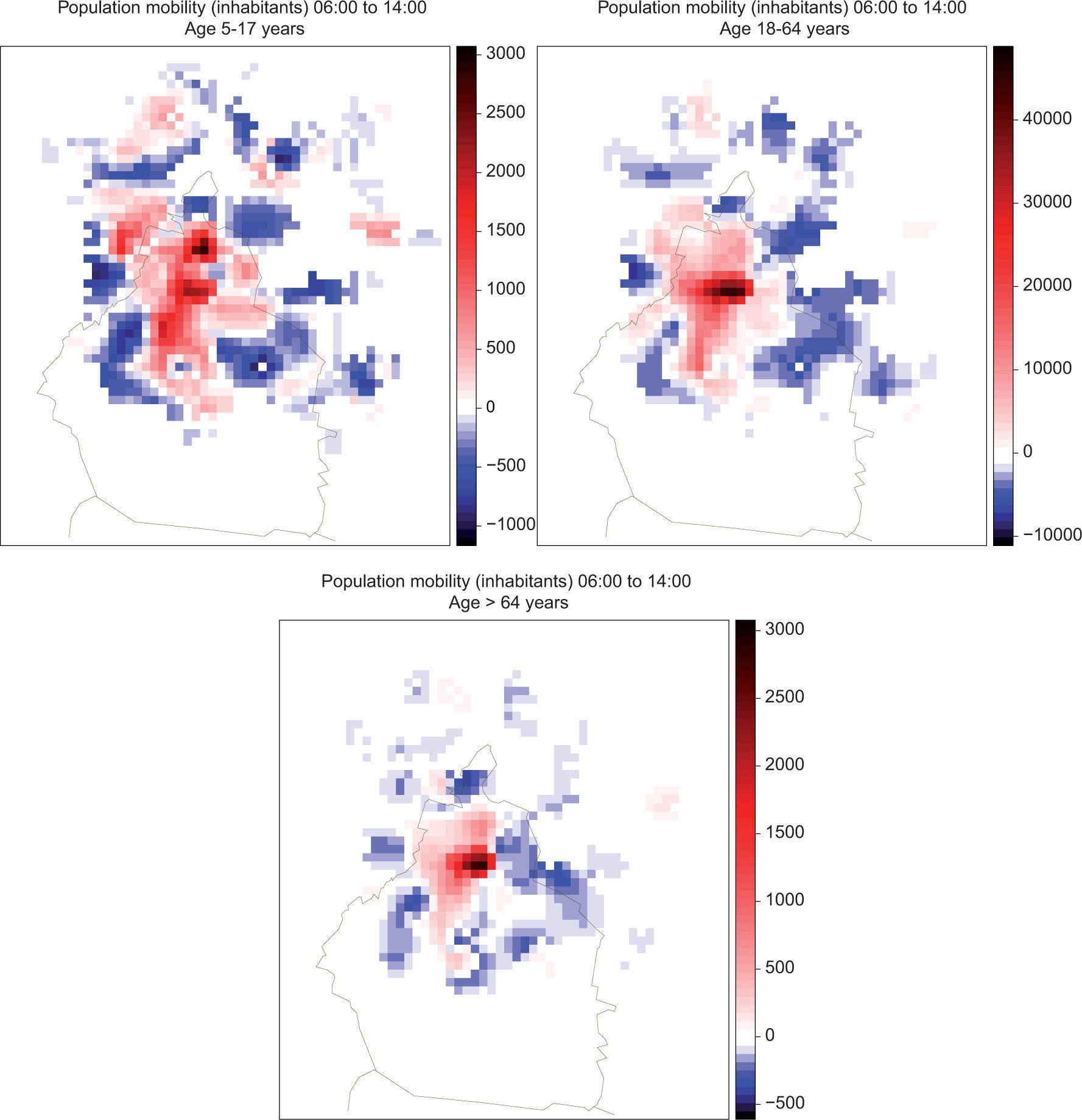
The differences for the spatial population distributions between 6:00 and 14:00 LT for a specific day of 2007 are plotted in Figure 2. Red pixels correspond to grid cells where population at 14:00 LT is greater than population at 6:00 LT, which we denote as incoming cells; while blue pixels correspond to grid cells where the population at 14:00 LT is smaller than the population at 6:00 LT, which we denote as outgoing cells.

Fig. 2.

Differences in population distributions between 06:00 and 14:00 LT, grouped by age.

Figure 2 suggests that working-age people (between 18 and 64 years) move more than younger and older people, while people older than 64 years have a relatively modest mobility.

In general, a pattern of increasing population in zones near the busy center of the city and decreasing population in peripheral zones can be observed. This pattern is more remarkable for the group of working-age people followed by the group of children and teenagers (from 5 to 17 years).

It is known that many people living in neighboring municipalities work or study in Mexico City, which explains such pattern. In this respect, some of the neighboring municipalities with outgoing regions are Naucalpan, Tlalnepantla, Atizapán de Zaragoza, Cuautitlán Izcalli, Tultitlán, Coacalco, Ecatepec, Nezahualcóyotl, Chimalhuacán, La Paz and Valle de Chalco.

5

Benefits estimation

In order to estimate the economical benefits in the HIA, the population-weighted ozone concentration C_PW for each hour t, given by the following formula, should be considered:

where P_ijt and C_ijt are the population and the ozone concentration in the (i, j) grid cell at hour t, respectively. C_PW(t) is a kind of spatial summary of concentration for hour t, where a weight proportional to its population is assigned to each cell.

This concept may be extended to a year, being the population-weighted concentration for year y, the maximum C_PW(t) among all the hours t of year y. Then, the following formula is used to estimate the number of avoided cases of an adverse health outcome during year y due to ozone reduction:

where P_y is the potentially affected population for year y, T_b is the base incidence rate (BIR) and is the concentration-response (CR) coefficient. The values presented in Table I for the parameters are considered in the evaluation of this formula. The number of avoided cases multiplied by the economic unitary valuation gives the economical benefit expressed in monetary units.

6

Results and discussion

For each cell in the population grid, the exposure corresponding to a given hour is estimated as the product of the number of people by the pollutant concentration in the cell. The unit of measure used is ppb × inhabitants; for example, an exposure of 10 000 ppb × inhabitants may be given by 100 people exposed to 100 ppb concentration of ozone. The maximum exposure for a year in a cell is computed as the maximum product of population by pollutant concentration in the cell over all the hours of the year.

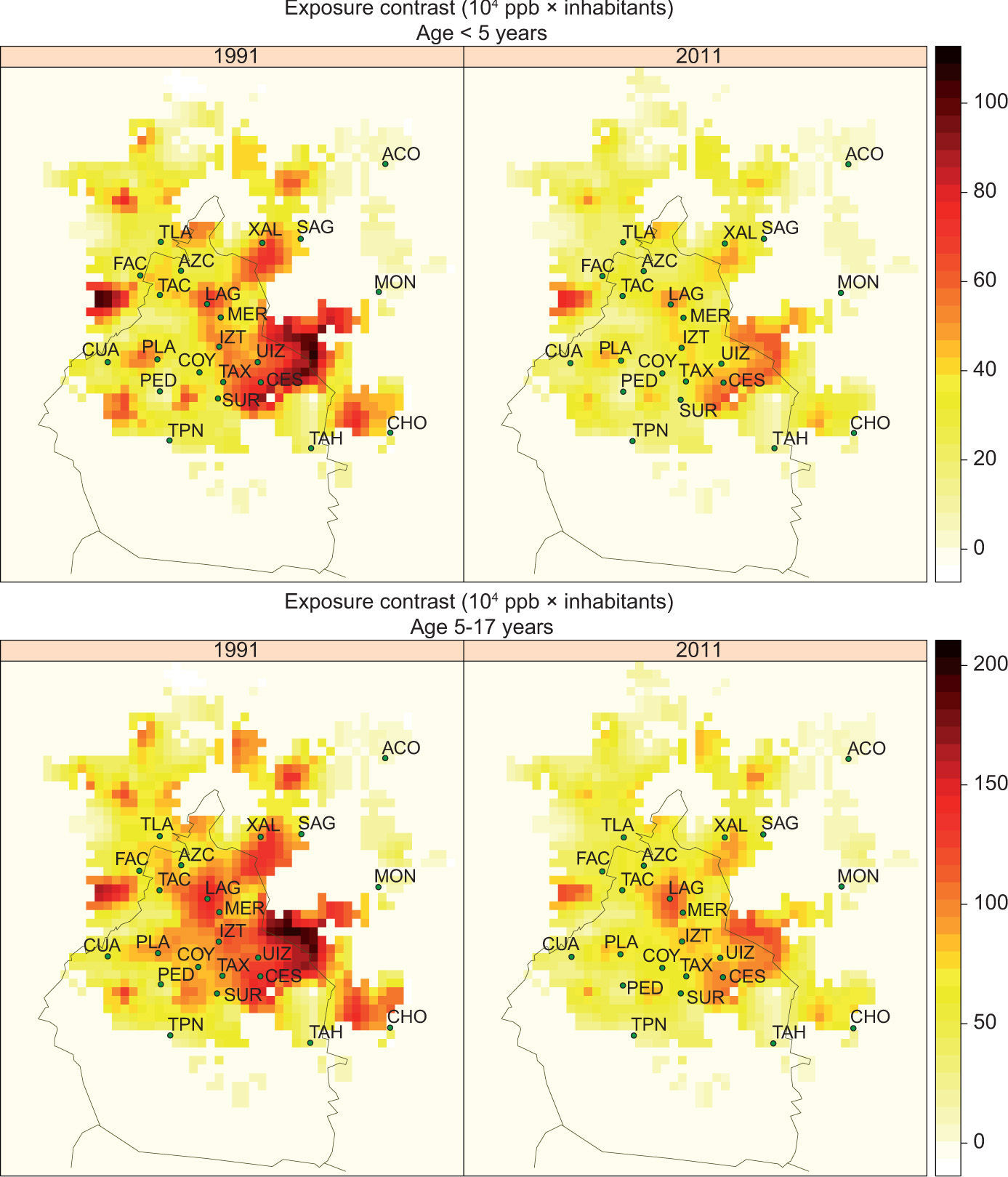
The maximum exposure maps for years 1991 and 2011 are shown in Figures 3 and 4, i.e. each pixel is colored according to the maximum exposure in the cell during the corresponding year. A map is presented for each population group. Figures 5 and 6 show the differences in such maps, i.e. the exposure reductions.

Fig. 3.

Potential exposure contrast, 1991-2011.

Fig. 4.

Potential exposure contrast, 1991-2011.

Fig. 5.

Yearly maximum exposure differences, 1991-2011.

Fig. 6.

Yearly maximum exposure differences, 1991-2011.

For children and teenagers (from 0 to 17 years), Figure 3 suggests exposures particularly acute in regions to the east and west of the central zone of the city during 1991, although the exposure conditions for such regions were still relevant during 2011. Fortunately, but not casually, the greater reductions in exposure have been achieved for these same regions with respect to the rest of the territory, as shown in Figure 5. In many cells the exposure has decreased to half or even less.

On the other hand, the groups of people of legal age (18 years or older) have a different spatial exposure pattern. For these groups, the central zone of the city and neighboring regions were the most affected areas during 1991, and continued to be so until 2011, as shown in Figure 4. Among these four groups, the most affected one is the group of working-age people, which has an exposure spatial pattern strongly focused around some kind of nucleus. Figure 6 also shows that greater reductions in exposure have been achieved for the most affected regions.

Figure 7 presents a bar plot for maxima of population-weighted ozone concentrations by population group, for three-year periods. As a consequence of ozone reduction policies, a decaying trend —simultaneous for every group— should be observed. Nevertheless, the values for the maximum population-weighted ozone concentration are still over 110 ppb, the threshold established by the Mexican Official Standard. Furthermore, a comparison between the periods 2006-2008 and 2009-2011 shows practically no differences.

Fig. 7.

Three-year population-weighted concentration maxima.

Table II shows the estimated total number of avoided cases by population group and adverse health outcomes from 1992 to 2011. In total, almost 2900 premature deaths were avoided, in addition to more than 11 100 hospital admissions for respiratory diseases, 3200 asthma attacks, 19 millions of MRAD and 35 million school loss days. The greatest number of avoided premature deaths, hospital admissions and MRAD was achieved for the group of working-age people. The other group considerably favored is the group of children and teenagers, particularly in the number of prevented school loss days (more than 35 million).

Table II.

Total number of avoided cases from 1992 to 2011.

	Population grouped by age				Total
	0-5	5-17	18-64	> 64
MORTALITY	294	603	1 801	197	2 897
RESP-HOSP	1 129	2 314	6 905	758	11 107
ASTHMA	1 060	2 173	-	-	3 233
MRAD	-	-	17 515 095	1 924 063	19 439 159
SCHOOL-LOSS	-	35 549 150	-	-	35 549 150

The groups of children less than 5 years old and people older than 64 years, considered particularly vulnerable to the damaging effect of pollutants like ozone, were not so favored as the rest of the population in the case of adverse health outcomes, which is worrisome.

Table III shows the estimated benefits in United States dollars (USD) of ozone reduction policies from 1992 to 2011. The economic valuation of the healthoutcomes is measured in USD from 2000 onwards, in order to compare the results with previous works.

Table III.

Total benefits in USD (2000) from 1992 to 2011.

Concept	Population grouped by age				Total
	0-5	5-17	18-64	>64
MORTALITY	88 373 952	181 099 448	540 465 817	59 371 096	869 310 314
RESP-HOSP	2 383 789	4 884 956	14 578 464	1 601 469	23 448 679
ASTHMA	336 174	688 902	-	-	1 025 076
MRAD	-	-	210 181 151	23 088 759	233 269 910
SCHOOL-LOSS	-	426 589 811	-	-	426 589 811
Total	91 093 916	613 263 118	765 225 433	84 061 325	1 553 643 793

The greatest economic benefits have been achieved by avoiding premature deaths, followed by school loss days and MRAD. With respect to age groups, the most favored were working-age people with more than 765 million USD, followed by the group of people aged 5 to 17 years, with more than 613 million USD.

The total benefits have been estimated in approximately $1.55 billion USD. This result contrasts with previous studies where population mobility was not regarded. Some of these studies yielded more than two billion USD (Huerta-Roldán, 2013). We explain this difference by the hypothesis that people move to less polluted regions during the day.

7

Conclusions

In this study, a health impact assessment for ozone reduction policies in Mexico City from 1991 to 2011 has been performed, taking into account the mobility of people during daytime, and interpolating ozone concentration data from monitoring stations to a regular grid by objective analysis. The studied population has been divided by age groups in order to contrast the results. It has been shown that different population groups have different spatial patterns of ozone exposure.

Working-age people have been the most favored by ozone reduction policies in terms of avoided cases and economic benefits, followed by the group of children and teenagers between 5 and 17 years of age. The groups of children less than 5-years old and people older than 64 years, considered particularly vulnerable to the damaging effect of pollutants like ozone, have been less favored in these terms. The former groups have higher mobility than the latter ones, which can be thought as a confirmation of the hypothesis that generally people move to less polluted regions during the day, which explains why greater benefits are achieved when a greater number of people moves.

This hypothesis has also been confirmed by the contrasting results yielded by previous studies where no population mobility was considered and benefits might have been overrated due to overestimations of ozone exposure and consequently of population-weighted ozone concentration.

The main contribution of this work is the particularization of the analysis for different population groups, regarding population mobility and the application of objective analysis in order to get spatially refined ozone concentration estimates.

7.1

Limitations

We recognize some limitations in this work, with emphasis in three aspects:

• •

  Population mobility spatial patterns.

• •

  HIA parameters.

• •

  The pollutant concentrations spatial interpolation method.

Firstly, we assume that spatial mobility patterns for each year are proportional to the ones yielded by the Encuesta Origen-Destino for Mexico City applied in 2007 (INEGI, 2007), adjusted by the total population in the given years. Furthermore, we assume that such patterns are the same for every day of the week and every month of the year, which is clearly unrealistic.

On the other hand, the considered HIA parameters represent just one choice among several available in the literature, because of the different approaches in their estimation.

Finally, there are methods for spatial interpolation more sophisticated than the Cressman objective analysis available in the literature. This method has been chosen because of its statement and implementation simplicity, and its relatively low computational complexity. In future works, other methods (such as spatio-temporal kriging or dynamic spatio-temporal hierarchical models) could be considered (Glover et al., 2008; Cressie, 1993; Cressie and Wikle, 2011; Sherman, 2011).

Acknowledgements

We would like to thank Dr. Arón D. Jazcilevich from the Centro de Ciencias de la Atmósfera and José M. Huerta from the Facultad de Química, both of the Universidad Nacional Autónoma de México (UNAM), for their relevant help and contribution to this research. We also acknowledge the financial support of the Consejo Nacional de Ciencia y Tecnología (Conacyt) for the fulfillment of this study.