Analysis of the hysteresis of unemployment in Mexico in the face of macroeconomic shocks

Abstract

This research presents the behavior of the Mexican unemployment rate and shows the dependence with own history and macro variables. The concept of hysteresis or persistence tries to separate this inertia in the unemployment rate and some macroeconomic and endogenous factors. The results show a high inertia in the Mexican labor market, justified by the monetary levels and the dependence of the investment levels, considering the shocks of exports that affect the unemployment in the long term.

Resumen

Este estudio expone el comportamiento de la tasa de desempleo para México y muestra la dependencia con su propia historia con variables macro. De esta manera se incorpora el concepto de histéresis o persistencia que intenta separar esta inercia en la tasa de desempleo y algunos determinantes macroeconómicos endógenos. Los resultados obtenidos muestran una inercia elevada en el mercado laboral mexicano, justificada por los niveles monetarios, así como la dependencia de los niveles de inversión, sin dejar de considerar que los shocks de las exportaciones afectan al desempleo en el largo plazo.

Introduction

When dealing with issues related to the uncertainty of economic agents, to analyze the macroeconomic variables through their historic evolution is usually of great interest; consequently, the making of decisions in economic policies is important. In this investigation, the main objective is to analyze the variable of Unemployment in Mexico through an econometric model, to determine in a real perspective the impacts on the behavior of the Mexican economy and its corresponding magnitudes in production, monetary offer and the external sector.

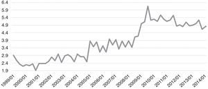
Based on the INEGI (2015) statistic that was analyzed, it is important to mention that in Mexico there has been a difficulty regarding the Unemployment variable to adjust to the levels observed between the year 2000 and before the global financial crisis of 2008; when it presented an average rate of 2.96% in each quarter.¹ Said situation has given rise to some questioning in the Mexican economy environment regarding the policies and plans of labor policies in the country, given the fact that in the last two presidential administrations, the average in the same temporal cuts of analysis, unemployment has been of 4.93%, i.e., higher by almost two percentage points, which reflects a lower labor stability for Mexican society in the long run.

The obvious importance of understanding the unemployment phenomenon in Mexico, lies in the characterization of the dynamic of the same in the face of the magnitude of the shocks that the Mexican economy is subject to in different stages of the economic cycle, taking into consideration the possible multiple balances and the memory of the behavior. With this it is possible to respond to the persistent behavior of the Unemployment issue, not only from the point of view of social protection and the labor reform recently implemented in the last two years, but also from the point of view of a macroeconomic stabilization policy.

The structural changes, reforms and low economic activity, compared to the persistent behavior of unemployment in Mexico, reflects an econometric analysis of great importance in order to determine the temporary effects with macroeconomic variables representative of the economic activity of the country. Economically defining the hysteresis in a time series, it is merely the long-term impact that remains in said series due to an endogenous or exogenous shock, i.e., a deviation due to an economic-structural change (Trejo & Vengas, 2010). Other investigations such as that of Wyplosz (1987), mention that this can be illustrated with the simple case of a dimensional linear discreet time system, in which the unemployment rate is subject to the lag of the variable and an error consideration or variables that are not considered in the system. Cross (1993) also mentions that more serious recessions could unchain answers that ensure that the current real unemployment rates have a persistent effect or even a permanent one on the balance rate. However, in light of the limited current economic literature that addresses hysteresis or temporal persistence in the Unemployment in Mexico, the search for its explanation is made interesting.

Recent investigations show, as is the case of Loria, De Jesús, and Jorge (2010), through a different approach, the search of an explanation for the recession and unemployment in Mexico from 1985 to 2009, a period during which the most important crises happened. Their investigation consisted in the extension of Okun's Law² for an open economy and with the incorporation of the productive gaps of the United States of America (USA), demonstrating that the aforementioned economy does not directly influence unemployment, so that the international transmission mechanism works basically through the production gap of the Gross Domestic Product of Mexico.

Another investigation that is not so recent but important for the basis of this investigation is the implementation for the Colombian case based on the model proposed by Maurer and Doris (1994), that signal the changes in some macroeconomic variables in order to demonstrate the existence of unemployment hysteresis in an economy. These investigators present the idea that the behavior of the unemployment rate strongly depends on its own history and is not easily explained by the aggregated demand or changes in the labor offer. Therefore, this situation of dependency is not captured in traditional models such as the Phillips Curve.

Therefore, in the econometric model developed in this investigation for the Mexican case, we expose a study with a temporary quarterly framework, considering the Unrestricted Vector Autoregressive methodology (UVAR) commonly used in the analysis of time series. Its application was done mainly to validate the effect relation between the endogenous variables, such as the internal economic activity reflected in the Gross Capital Formation (GCF), or the consideration of the degree of relation with the external sector through the levels of Exportation (EX); without casting aside the internal activity or liquidity through the increases of the Basic Monetary Aggregate (M1).

For the proposal of a UVAR model for Unemployment in Mexico, a statistical analysis was done in order to explain the historic evolution of the endogenous macroeconomic variables. This allowed for the analysis of the existence of stationarity, in order to identify the different levels in which these variables may be used to measure in time the shocks that affect the Unemployment variable. The selection of a UVAR model is presented in the work based on the results obtained with the Box Jenkins technique and the methodology of Johansen, which indicate that there is no co-integration in the long-term. Furthermore, econometric measures of normality, autocorrelation and heteroscedasticity in UVAR terms were implemented in order to guarantee the existence of an Unemployment hysteresis in Mexico.

The document is divided as follows. In the first section, we do a theoretical and literary review regarding the level of unemployment and the hysteresis of the same, considering the source of the data used as endogenous variables. While in section two, we evaluate the macroeconomic performance and the labor market in Mexico. In the third section, we apply econometric techniques to identify the UVAR model. Finally, we present the main conclusions of the investigation.

Background and data used

The concept of hysteresis has, as its main objective, to separate the level of inertia of the unemployment rate and its macroeconomic determinants. The use of the term hysteresis or persistency in economy, has been used by Phelps (1972), Blanchard and Summers (1986) and Lindbeck and Snower (1986). It has also been used in the foreign trade theory, see the work of Baldwin and Krugman (1989), Dixit (1989), Dias and Shakleton (2005). For the analysis of prices and their shocks in time for the Mexican case, Trejo and Vengas (2010) proposed the implementation of the persistence or inflationary hysteresis in time windows on the same inflation.

The main representation of hysteresis is based on the Mayergoyz (1986) model, who proposed a magnetic hysteresis model, which is used as reference in order to perform an analysis of foreign trade and of the labor market, due to the clear use of said concept. This implementation can be seen in microeconomic and macroeconomic works, see Amable, Henry, Lordon, and Topol (1995), Cross (1987, 1993), Göcke (2002), and the applications in the Mayergoyz model (1991).

There are some hypotheses on the incorporation of hysteresis in the labor market due to the deficiency that exists in the Phillips Curve, proposed by the economist William Phillips in 1958.³ The long-term focus that was proposed and the relation that exists between the natural rate of unemployment (NRU),⁴ in theory, converge at the balance of some events that cast doubt on this relation, as during the seventies the high levels of inflation and the rate of unemployment ended this relation. Therefore, it is necessary to evaluate the unemployment rate against the variation of inflation.

The traditional analysis of employment presents the idea that unemployment is affected by some exogenous factors in the long-term (prices of productive and technological factors, etc.). Whereas in the short-term, the changes occur on the offer and demand, generating a deviation with regard to the natural unemployment. The immediate impacts in the inflation rate do not have an effect in the long-term with the return of unemployment to the original balance, so that the relation with the economic growth and the natural rate of unemployment is also clear.

There are works that analyze the relation between the product and employment, stating that unemployment has great social and economic inter-temporal costs that cause long-term negative effects, in addition to repeating themselves continuously. Some empirical studies try to observe if the unemployment level maintains some tendency in the periods subsequent to the shocks caused by economic policies or other random factors that have a repercussion in the system (Gordon, 1989).

However, recent investigations that show a relation in the hypothesis of hysteresis explain that the fluctuations in the economy could permanently affect unemployment due to the rigidity of the labor market; this hypothesis shows that the unemployment rate follows a non-stationary process with a unit root (Blanchard & Summers, 1991).

Due to the above, this investigation also aims to analyze the behavior of the Unemployment rate in Mexico, with its own history through a new analysis framework, this due to the fact that the traditional model of the Phillips Curve does not capture this dependency, inserting the concept of hysteresis that seeks to separate this inertia in the unemployment rate and some macroeconomic determinants.

To economically define hysteresis in a temporary series, it is simply the long-term impact that prevails in said series duo to an endogenous or exogenous shock, i.e., a deviation due to an economic change. The origin of hysteresis comes from the natural sciences that reflect the fact that after the causes that generate a certain event have disappeared, the situation does not go back to its original state, rather, the phenomenon remains in time or, in other words, it persists (Trejo & Vengas, 2010).

In order to evaluate the evolution of unemployment hysteresis in Mexico, it is necessary to operationally consider that it is not only the inertia of past events of the same unemployment variable, but also of other structural macroeconomic variables, such as the ones coming from the monetary sector, foreign trade and the national productive activity. The persistence of unemployment is related in this document to the velocity in which a shock of behavior of the same variable, as well as that of macroeconomic variables, affects Unemployment in the future. This notion of persistence is what is traditionally defined for stationary time series.

The application for the Mexican case is to evaluate the impact of four endogenous macroeconomic variables for that of the labor market. The study was carried out with quarterly data from the first quarter of 1999 to the fourth quarter of 2014, given the availability of data.

Table 1.

Variables to be estimated in the econometric model.

Variable	Description
DES	It is unemployment.
M1	It is the money supply. Includes bills and coins as well as checking accounts in national and foreign currency held by all economic agents.
FBK	Capital formation.
EXP	Son las exportaciones de bienes y servicios

Source: Own elaboration, with definitions of the Bank of Economic Information (BIE), INEGI (2015).

Macroeconomic performance and labor market in Mexico

It is important to mention that the unemployment rate in Mexico was one of the lowest in the world 14 years ago. According to data from the World Bank, in 2000 Mexico was one of the seven nations with the lowest rate (2%), when there were other countries with very high rates, 39.3% in Lesotho, 34.5% in Macedonia, 28.7% in Algeria, 25.7% in Yugoslavia, even so lower than in some industrialized countries such as France 10%, Germany 8.1%, Italy 10.8%, Spain 14.1% and the United States 4.1% (Liquitaya & Lizarazu, 2005).

This discrepancy that exists in the different rates could be justified by the way of measuring the unemployment rate in Mexico. The methodology used sticks to the recommendations of the International Labor Organization (ILO), when defining the economically active population (EAP) that comprises everyone above 14 years for the INEGI, whereas in Germany it comprises everyone above 15 years, Italy 14 years, Spain, USA and France, 16 years. This aspect does not produce a decrease in the rate of Mexican unemployment, conversely, it generates an increase due to the proportion of unemployed people in the lower age range and which is more elevated for the people in the upper age range, as it is mentioned by Fleck and Sorrentino (1994) and Hernández, Garro, and Llamas (1997).

In Mexico, since 1998, there has been debate on the need to make labor policies more flexible. With the implementation of the NAFTA, this necessity increased due to the new global context of the market and the production, the modernization of the market in certain productive processes, as well as the need to provide more reliability to the investors, and the need to elevate productivity and quality. Due to this, the labor policy suggests a reform with the objective of elevating productivity and quality in the same productive apparatus. Other factors such as the depreciation of human capital, stimulated by long periods of unemployment, the lack of innovation and the asymmetric information can generate hysteresis, making it even more complicated for the rate of unemployment to go down, even in period of economic boom (Maurer & Doris, 1994).

The periods during which an increase of unemployment arises and there is persistence of the same, is not a rare event throughout history, and people have had a hard time explaining it. Some authors such as Blanchard and Summers (1987) argue that such a phenomenon should be understood in terms of the hysteresis that it generates, which in the long-term the balance depends on its history.

Unemployment in Mexico

The importance of the unemployment rate in Mexico turns out to be a very important indicator for the evaluation of the economic performance of a country, thus the interest given to the analysis of the role that it plays in the Mexican economy. According to the results of the Encuesta Nacional de Empleo (ENOE) (National Employment Survey), at the closure of 2014, 59.86% (participation rate) of the population in working age (not of 14 years but above 15 years, given the recent constitutional reform that added a year to the minimum working age) was economically active (EAP, people employed or looking for employment), a lower percentage than the one of the previous year (61.08%). 96.24% of the EAP was identified as Working population (WP), which means that the unemployment rate (UR) was of 3.76% in December (against the 4.53% in November, the 4.27% a year before and the 4.20% expected), decreasing for the fifth month in a row and situating itself at its lowest level in at least two years. Thus, the average UR of 2014 was of 4.83%, lower to the 4.91% of 2013.

The good result of the unemployment rate in December of 2014 coincides with the favorable end in matters of formal employment generation, as the number of insured workers in the IMSS (despite its usual setback of the last month of each year) was lower than the one of 2013, while its growth rate improved from 4.2% to 4.3%, being the most dynamic since January 2013. This reflected an improvement in the rhythm of economic activity in the last quarter of 2014 that, should it extend to 2015, should contribute to keeping a labor dynamism that is at least similar to that at the closure of 2014.

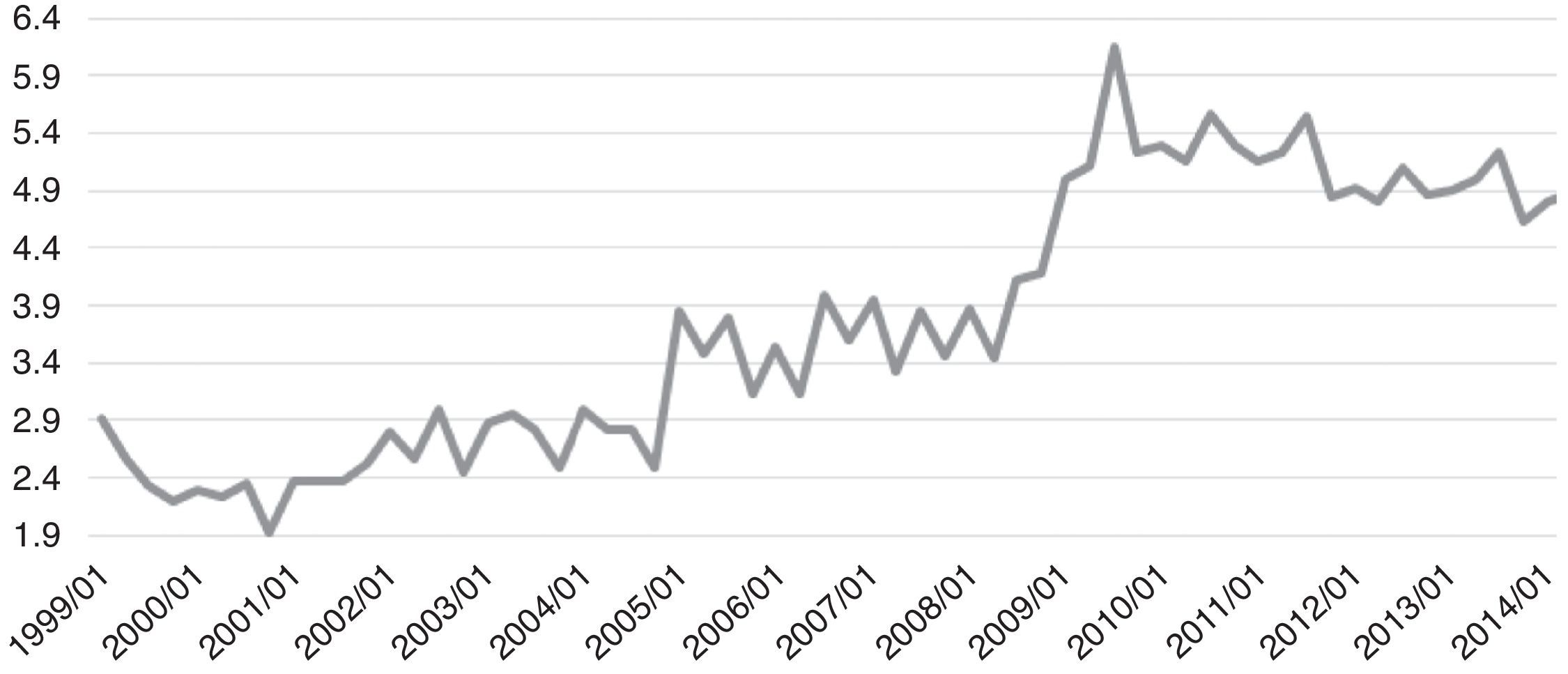
Fig. 1 shows the evolution of the unemployment rate from 1999 to 2014, in which the last 14 years presents an upward trend and a break with regard to the tendency after the peak of the unemployment rate (6.15) reached in 2009, this as a consequence of the global liquidity crisis. The slight decrease of rates in the last five years is due to the scarce economic activity in Mexico, with annual economic growths inferior to 3% after the last world crisis and to the labor reform implemented in the current presidential administration. This coincides with the favorable year closure with regard to the creation of formal employment and to an improvement in the economic activity rhythm at the end of 2014. Should this behavior continue in 2015, it would contribute to keeping a labor dynamism that is at least similar to the closure of 2014.

Performance of the gross capital formation in Mexico

In all economic investigations related to the economic growth of a country, the GCF investment is a determining factor in the representation of the engine that boosts an economy forward. From the beginning of the 1980s, investment in Mexico, as with the rest of the world, has been defined with regard to the conditions that the financial globalization imposes. However, Mexico has not managed to establish a favorable dynamism regarding the accumulation of capital that allows experiencing a vigorous growth rhythm. This situation has been analyzed by Avendaño and Perrotini (2015), who argue that the growth of the GCF has been insufficient to absorb the labor force of the economy.

In Mexico, from the 2000 to 2008, the investment component of the GCF presented a stage of growth that was stalled by the effects of the global liquidity crisis, which caused a growth rate of 9.75% between 2008 and 2009. While since 2010 to the closure of 2014, the GCF has only had a quarterly mean growth of only 2.81%, demonstrating the low levels of dynamism and the lack of economic growth in Mexico.

The GCF variable that is comprised in the record on the expenses made in national and imported machinery and equipment, as well as those resources that were used to develop residential and non-residential constructions, reported a growth of 5.7% at an annual rate reported in 2013 of −4.8%, with this figure being positive since its peak in May 2014.

In the aggregate, the balance that the GCF presents in September has a moderately positive slant, particularly due to the peak regarding the decreases recorded since 2012; within this comparison, the component of machinery and equipment that evolves with greater dynamism than construction, stands out; in spite of this, this impulse is still not consistent enough with the rhythm of industrial production, forcefully linking us to the decreasing vigor in the demand of the internal market. On the other hand, even if the investment in construction has shown a boost in recent years according to its annual rate (particularly in residential construction), this has not had the sufficient strength to revert the negative figures in the annual variation accumulated for more than two years.

Exports in Mexico and their compositions

At the closure of 2014, the commercial balance in Mexico recorded a surplus of 254 million dollars (md), same that was lesser to the one in the previous year (1626 md) and contrary to November's deficit (−1076 md). This result originated from a vigorous annual acceleration of exports, from 2.1% to 6.4%, same as with imports, from 6.5% to 11.2%.

In the composition of last year's exports, it was emphasized that the oil companies notoriously accented their annual deterioration rate, from −13.2% in 2013 to −43.7% in 2014, while the non-petroleum companies significantly improved their advance, from 4.0% to 14.3%, with manufacturing companies going from 4.0% to 15.8% in 2013 and 2014 respectively.

Regarding the destination of the manufacturing sector, the exports that go to the USA accelerated their growth from 6.3% to 16.2% annually and toward the rest of the world from −5.2% to 6.2%. However, the commercial balance of all of 2014 was a deficit of 2441 million dollars, higher than the one observed in 2013, when it was of 1184 million dollars, with external sales reporting an accumulated increase of 4.6% and the foreign purchases of 4.9% (in light of increases of 2.5% and 2.8%, respectively, a year before).

If the United States economy remains this solid and the recovery rhythm of the economic activity and the consumption levels in Mexico improves, the export and import dynamism will continue to improve. Although, it should not be overlooked that as long as the prices of oil do not recover and the structural reform of the energy sector is not implemented, creating more investments in the sector, this will continue to be reflected in the low levels of oil exports.

Importance of the monetary aggregate (M1) as financial stabilizer in Mexico

In Mexico, the monetary policy has as its main objective to maintain inflation stable. However, said policy has effects on unemployment. The monetary policies link these variables, and therefore require a prediction of the effect that a change in these would have and the quantity of money or interest rate on unemployment in order to establish a more accurate monetary policy.

For the closure of 2014, the monetary policy showed the need to strengthen the macroeconomic framework in the face of a highly uncertain and complicated global financial environment. In the USA, the economy continued to consolidate its recovery with the strengthening of the global market, and the Federal Reserve of the USA withdrew its normalization plans in its monetary stance. Whereas in the case of Mexico, the economic activity showed a moderate recovery, with the external sector being the main trigger of the growth, combined with a greater dynamism in private investment, however, with uncertainty of lesser levels of growth than those predicted.

Macroeconomic context in Mexico

Generally, the behavior of the prices of petroleum and explained in the degree of exports, combined with the management of possible increases in interest rates in the USA at the closure of 2014, reflected a less expansive macroeconomic stance. In Mexico, the total employment is still weak at the closure of 2014 in spite of the expansion of formal employment, and the real total payroll continues to decrease, which causes an obstruction in consumption. Lower petroleum prices could reflect the reduction of profitability of the projects that would result from the energy reform; and with this, a decrease on the effects of the daily economic activity. There is the risk that other structural reforms, such as that of competition, do not have the expected result. In addition to the aforementioned, the broad deficit of the non-petroleum commercial balance could imply a risk of a financing shock in the economy that would impact a rise in inflation.

The macroeconomic environment that the Mexican economy faced at the closure of 2014 generated pressures on the real exchange rate and the interest rates, and thus in this context the fiscal policy must be an anchor in order to be able to absorb said pressures in an orderly fashion. It is urgent to stabilize the growth of the financial requirements of the public sector, which have gone from 26% of the GDP in 2006 to 42% of the GDP at the closure of 2014. Therefore, the monetary policy always plays a rather important role in facing the external environment, for the anchoring of the expectations of inflation and in order to prevent a disorderly displacement in the yield curve.

The increases in the prices of high-calorie foodstuff that came about as consequence of the new tax implemented in 2013. The inflation at the closure of 2014 was found to be above 4% in good measure by transitory effects such as these.

For 2015, many of these effects will disappear, and there will be other factors that ought to help for a quick decline of inflation such as, for example, the manner in which the elimination of fees in telecommunications is measured, such is the case of the long-distance fees. These types of effects are also transitory, and thus, it should not be thought that inflation is already fully complying with the goal. There are other factors whose possible evolution is still unknown, but that could have a rather significant effect on inflation, such as a significant increase in the minimum wage or the permanence of the high levels in the exchange rate. Considering that the Federal Reserve of the USA appears to be in line with a first increase of its interest rates toward the middle of the year, and in the face of the high probability of it becoming a reality, during the first half of the year, an increase in the minimum wage above the expected inflation and of the expected earnings in productivity; we can conclude that it would be during the middle of 2015 when Banxico begins to raise its reference interest rate.

Identification of the unrestricted VAR model for unemployment

The econometric estimations implemented in this investigation in order to understand the behavior of unemployment in Mexico from 1999 to 2014, are based in vector autoregressive models without restrictions, given the lack of co-integration in the long-term of the independent variables (EX, GCF, and M1) with the dependent variable (DES).

Therefore, diverse econometric tests are required in order to sustain that with a minimum of restrictions, the proposed model is operational for the case of unemployment in Mexico.

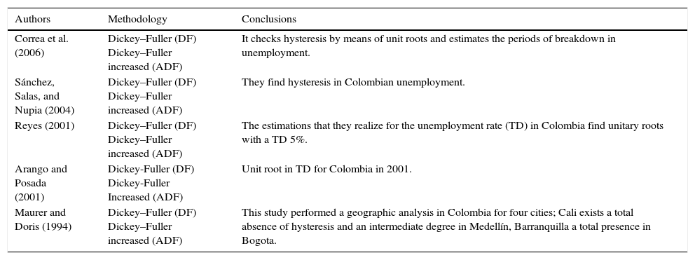
Table 2 shows some investigations on the hysteresis that have implemented the unit root methodology in order to prove the existence of pure hysteresis I(1), therefore, this data generating process is characterized by having infinite memory, which means that the unemployment rate could be highly correlated with its past.

Table 2.

Estimation of hysteresis through unit roots.

Authors	Methodology	Conclusions
Correa et al. (2006)	Dickey–Fuller (DF) Dickey–Fuller increased (ADF)	It checks hysteresis by means of unit roots and estimates the periods of breakdown in unemployment.
Sánchez, Salas, and Nupia (2004)	Dickey–Fuller (DF) Dickey–Fuller increased (ADF)	They find hysteresis in Colombian unemployment.
Reyes (2001)	Dickey–Fuller (DF) Dickey–Fuller increased (ADF)	The estimations that they realize for the unemployment rate (TD) in Colombia find unitary roots with a TD 5%.
Arango and Posada (2001)	Dickey-Fuller (DF) Dickey-Fuller Increased (ADF)	Unit root in TD for Colombia in 2001.
Maurer and Doris (1994)	Dickey–Fuller (DF) Dickey–Fuller increased (ADF)	This study performed a geographic analysis in Colombia for four cities; Cali exists a total absence of hysteresis and an intermediate degree in Medellín, Barranquilla a total presence in Bogota.

Source: Extracted from Correa, Castro, Bríñez, and Posso (2006).

Stationarity tests of the endogenous variables

Based on the results obtained and seen in the multiple balances of unemployment, we can affirm that the reforms meant to reduce the extra labor benefits could constitute important positive shocks if implemented in the employment recovery phase, thus reducing the unemployment rates (Aranda, 2003). However, when the reforms are implemented in periods of growing unemployment, these cannot have the desired effect due to the fact that the potential beneficial effect of the reform is offset by a negative shock (Monetary Offer and Exports) that affects the economy.

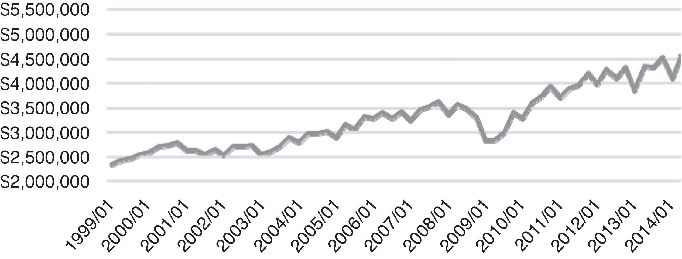
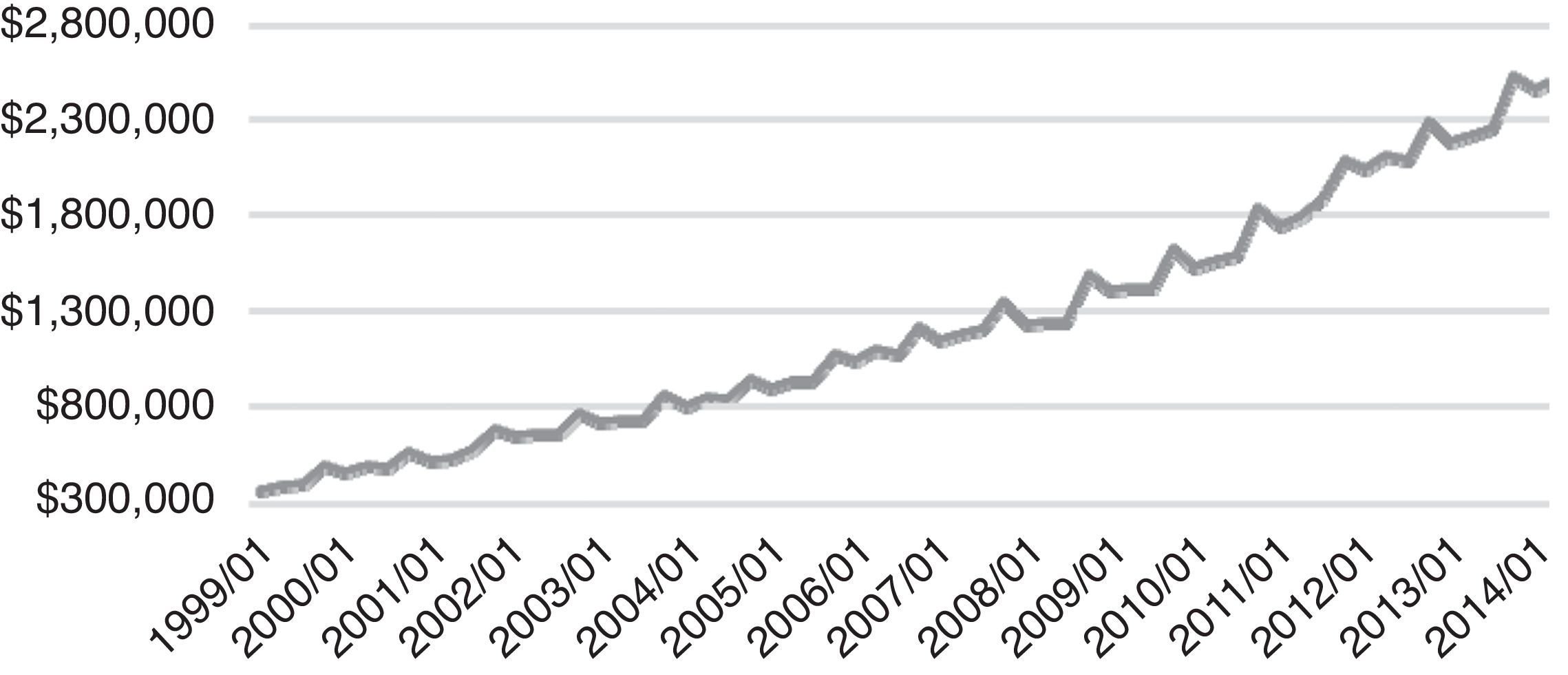
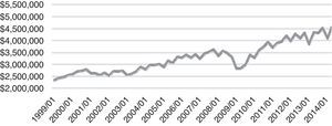
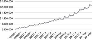
Within the temporal evolution analysis of the variables used, it can be observed in Figs. 1–4, that the behavior of the series empirically shows a lack of stationarity based on the reflection of growths and tendencies.

Fig. 1.

Quarterly unemployment rate 2000–2014.

Source: own elaboration with data obtained from INEGI (2015).

Fig. 2.

Quarterly gross capital formation 1999–2014 (million pesos).

Source: Own elaboration with data obtained from INEGI (2015).

Fig. 3.

Quarterly exports 1999–2014 (millions of pesos).

Source: Own elaboration with data obtained from INEGI (2015).

Fig. 4.

Monetary aggregate M1 quarterly 1999–2014 (millions of pesos).

Source: Own elaboration with data obtained from INEGI (2015).

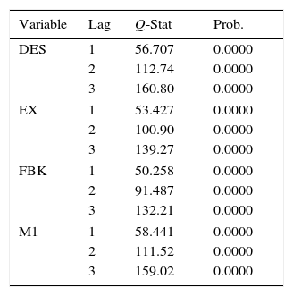
With the purpose of modeling the behavior in time by means of autoregressive techniques, it was considered to transform said independent variables (FMK, M1, and EXP) into logarithmic variables, homologizing the characteristics of econometric analysis with the Unemployment variable. An analysis carried out in order to corroborate the existence of stationarity, was the validation of the correlograms of each of the series (Table 3).

Table 3.

Correlogram and stationary.

Variable	Lag	Q-Stat	Prob.
DES	1	56.707	0.0000
	2	112.74	0.0000
	3	160.80	0.0000
EX	1	53.427	0.0000
	2	100.90	0.0000
	3	139.27	0.0000
FBK	1	50.258	0.0000
	2	91.487	0.0000
	3	132.21	0.0000
M1	1	58.441	0.0000
	2	111.52	0.0000
	3	159.02	0.0000

Source: Own elaboration with 64 quarterly data obtained from INEGI (2015), up to 8 delays (quarterly) and the use of the econometric analysis package of Eviews8.

Through a difference, that is, integration of the first order I(1), it allows the identification of the linear combination of stationarity. Its representation is found with a “D” in each variable: DDES, DEX, DGCF, and DM1. In order to explain the evolution of the series in the course of time and predict its future values, it was required to validate the transformation of non-stationary variables to stationary variables, i.e., proof the effectiveness of the elimination of tendency and heteroscedasticity through the differentiation 1 (Table 4).

Table 4.

Unit root testing.

Variable	No difference ADF t-statistic	p-value (5%)	Type of series	With 1 difference ADF t-statistic	p-value (5%)	Type of series
Unemployment	−1.445368	0.5540	Not Stationary	−3.458677	0.0127	Stationary
Exports	0.334835	0.9782	Not Stationary	−4.807410	0.0002	Stationary
Gross capital formation	−0.717168	0.8341	Not Stationary	−3.708960	0.0130	Stationary
Monetary attachment M1	−0.955910	0.7632	Not Stationary	−3.473728	0.0122	Stationary

Source: Own elaboration with 64 quarterly data obtained from INEGI (2015) and to the use of the package of econometric analysis of Eviews8.

Only one lag was used and variables in logarithm, which represents a generalized consideration of variables per quarter. This allows the validation of the autocorrelation of the residuals and thus the necessary parsimony, in the sense of not including an excessive number of lags. Therefore, it is thought that the series considered would be integrated of the first order I(1) and the first differences would be stationary.

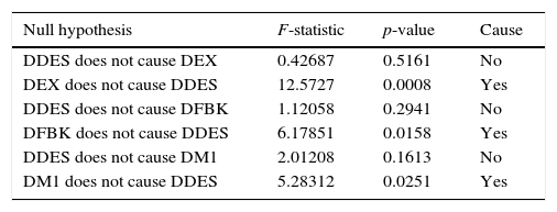
Causality of macroeconomic variables with unemployment in Mexico

In order to describe and infer in the causal dynamic between unemployment and the endogenous macroeconomic variables mentioned, based on the autoregressive vector models, Table 5 can be validated.

Table 5.

Granger Causation Test (1969), 1999Q1–2014Q4.

Null hypothesis	F-statistic	p-value	Cause
DDES does not cause DEX	0.42687	0.5161	No
DEX does not cause DDES	12.5727	0.0008	Yes
DDES does not cause DFBK	1.12058	0.2941	No
DFBK does not cause DDES	6.17851	0.0158	Yes
DDES does not cause DM1	2.01208	0.1613	No
DM1 does not cause DDES	5.28312	0.0251	Yes

Source: Own elaboration with quarterly data obtained from INEGI (2015) and to the use of the package of econometric analysis of Eviews8.

In this way, it is detected that it complies with the modeling principles required in this investigation; first the independent variables (endogenous) cause the unemployment variable, in addition to avoiding problems of reciprocal correspondence.

Long-term co-integration test of endogenous variables

Given a group of non-stationary endogenous variables, it was of interest to determine if the series are co-integrable or not with unemployment, and if they were, identify the co-integration relations in the long-term balance. The methodology used in this type of analysis was the Johansen method, considering a VAR with order p; y_t = A₁y_t−1 + ⋯ + A_py_t−p + Bx_t + E_t, where y_t is a k-vector of the non-stationary contemporary endogenous variables mentioned (DES, DEX, DGCF, and DM1) I(1), y_t−1 vector of aforementioned endogenous variables, lagged one period, x_t is a d-vector of deterministic variables, A_i matrices of coefficients of regression to be estimated for i = 1,2,…,p and E_t is a vector of innovations, which are assumed as not serially correlated.

Therefore, in this case the Vector Error Correction Model (VECM) cannot be used, thus opting for analyzing a UVAR system (Table 6).

Table 6.

Johansen cointegration test 1999Q1–2014Q4.

Number of cointegrated equations	Trace statistic	0.05 critical value	Prob.	Max-eigen statistic	0.05 critical value	Prob.
Neither	11.45	15.5	0.19	10.97	14.27	0.16
At least 1	0.47	3.84	0.49	0.48	3.84	0.49

Source: Own elaboration with 61 quarterly data after adjustments and obtained from INEGI (2015), up to 1 delay and with the use of the econometric analysis package of Eviews8.

The unrestricted VAR model

The model implemented for the Mexican case takes the model proposed by Maurer and Doris (1994) as reference, which describes the changes in some macroeconomic variables in order to demonstrate the existence of hysteresis. Thus, the model proposed is expressed as follows:

where α_t: unemployment in period t; λ: the fraction of unemployment for the period t − 1; Z_t: some endogenous macroeconomic variables in time t and A: weight coefficient.

It is important to mention that in the model, due to the existence of memory, the effects of a policy reflected by variable Z weighted by coefficient a transfer to unemployment time t or present.

In hysteresis, unemployment in the current period t is exactly equal to period t − 1, though it ought to be clarified in the case that there are no other factors that exercise influence on it. The general definition of hysteresis refers to the persistence or inertia, so that for unemployment during a period it shall be a fraction λ of the previous unemployment; these values are between 0 and 1 and indicate a strong or weak persistence. A λ value greater than 1 would make no sense as it indicates an explosive amplification of unemployment; a λ value equal to zero indicates the absence of an intertemporal process of unemployment.

The unrestricted autoregressive vector, UVAR, is obtained given a number of delays, with the representation I(1) obtained in Table 1. The qualifier “unrestricted” reflects the fact that the UVAR model incorporates a minimum of restrictions necessary to be operational.

The UVAR model has been highly used in the applications of the VAR methodology. On the one hand, due to its broad generality as an instrument to represent stochastic processes and, on the other, its easy estimation through methods with adequate statistic properties, such as the method of ordinary least squares (OLS). This method possesses a normal asymptotic distribution, being the most efficient unbiased linear estimator. Thus, in the UVAR framework, we look for unemployment to have stochastic and non-deterministic regressors as it occurs with the simple linear regression, in addition to the fact that the vector of disturbances is present in a succession of random independent vectors, without autocorrelation between the current value of disturbance and the regressors of the model.

Based on the analyses of Maurer and Doris (1994), considering the analyses of the temporal series in previous sections, an equation that explains the effect of hysteresis in the labor market in Mexico is suggested.

Through a linear model of the five variables determined in Eq. (2), the behavior of Unemployment in Mexico can be explained by its very own lagged values in a quarter, determined with the unit root tests and with the causality tests. Thus, the UVAR model can predict the interrelated system of the series of time in order to measure the dynamic impact with the dependent variable with random disturbances.

Econometric diagnostic of UVAR

The optimal lag for the modeling was determined through the Schwartz Criteria, which indicates that with a minimum value of −9.51, a lag is sufficient (Table 7).

Table 7.

Selection criteria with order of lags VAR 1999Q1–2014Q4.

Lag	Log L	LR	FPE	AIC	SC	HQ
0	240.7163	NA	3.35e−09	−8.162632	−8.020532	−8.107281
1	299.2906	107.0495	7.73e−10	−9.630710	−9.518623^a	−9.353957
2	349.1281	84.20814	2.43e−10	−10.79752	−8.920212	−10.29936

a

Indicates the selection criteria of the lag order.

LR: sequential modified LR test statistic (each test at level 5%), FPE: final prediction error, AIC: Akaike information criterion, SC: Schwarz information criterion, HQ: Hannan–Quinn information criterion.

Source: Own elaboration with 61 quarterly data after adjustments and obtained from INEGI (2015), up to 1 delay and with the use of the econometric analysis package of Eviews8.

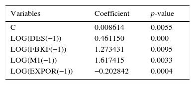
Table 8 shows the results of the econometric estimation of the model.

Table 8.

Estimation of the UVAR econometric model.

Variables	Coefficient	p-value
C	0.008614	0.0055
LOG(DES(−1))	0.461150	0.000
LOG(FBKF(−1))	1.273431	0.0095
LOG(M1(−1))	1.617415	0.0033
LOG(EXPOR(−1))	−0.202842	0.0004

Source: Own elaboration with data obtained from Bank of Mexico and with the use of the package of econometric analysis of Eviews8.

The results of the estimation of the model show that all the variables are statistically significant. Furthermore, the model has a goodness of fit of 85% and the Durbin–Watson (1971) statistic shows the absence of autocorrelation. The value obtained for unemployment is found in a range of 0 > 78 < 1, thus there is persistence considering these variables. The estimations carried out by López (1993) base their analysis on a random function based on the Weibull distribution⁵ and the insertion time in the labor market of an unemployed person, the time scheme goes from one to twelve months, and it also shows that there is a relation between the probability that an unemployed person has of entering into the market with the market and the hysteresis coefficient.

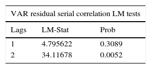
Autocorrelation

The Breusch (1978) and Godfrey (1978) test was carried out in order to detect the presence of serial dependence, as if that is the case, the conclusions are incorrect (Table 9).

Table 9.

Autocorrelation test (Breusch–Godfrey).

Breusch–Godfrey serial correlation LM test
F-statistic	0.977008	Prob. F(1,56)	0.3272
Obs * R-squared	1.063139	Prob. Chi-square(1)	0.3025

Source: Own elaboration with the use of the econometric analysis package of Eviews8.

The correlations between combinations of endogenous and lagged variables of the model did not show problems of autocorrelation. If the aforementioned is corrected, then the VAR model determined for the estimation of Unemployment must not have any residual autocorrelation.

In Table 10, we can observe that the p-value is equal to zero, indicating that there is no Serial Correlation and thus the terms of error within the model of unemployment are consistent.

Table 10.

Residual correlation test VAR (LM test).

VAR residual serial correlation LM tests
Lags	LM-Stat	Prob
1	4.795622	0.3089
2	34.11678	0.0052

Source: Own elaboration with the use of the econometric analysis package of Eviews8.

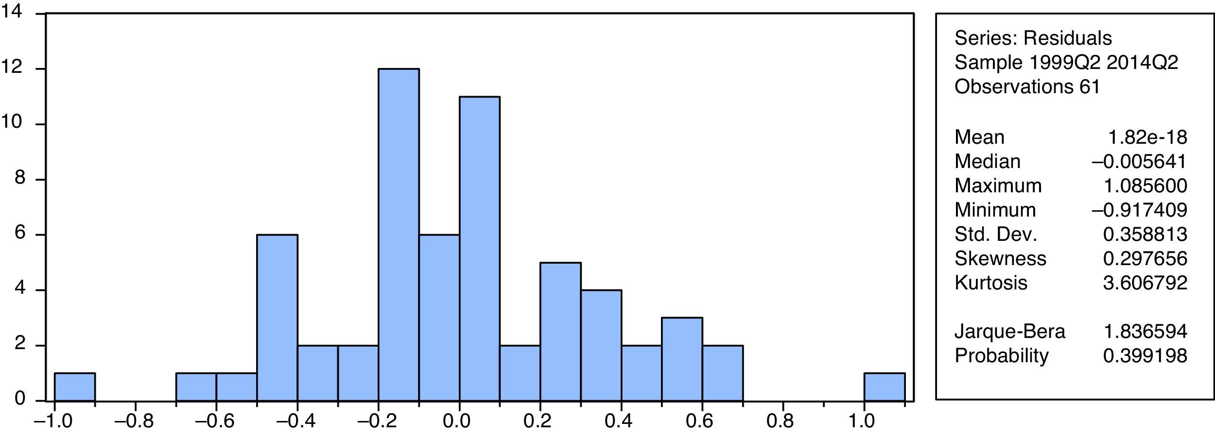
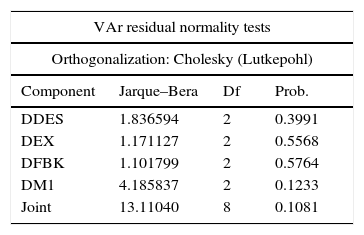
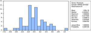
Normality

Though a statistic process to determine if the data could adjust to a normal standard distribution, the residuals of the UVAR model of Unemployment showed a distribution with a median of zero and a constant variance. Nevertheless, Fernandez-Corugedo, Price, and Blake (2003) argues that it is more important that the UVAR complies with the no autocorrelation test of errors than with the multivariate normality. However, through the Choleskey (Lutkepohl, 2005) text, the normality of the proposed Unemployment model was validated (Table 11).

Table 11.

Residual normality test VAR.

VAr residual normality tests
Orthogonalization: Cholesky (Lutkepohl)
Component	Jarque–Bera	Df	Prob.
DDES	1.836594	2	0.3991
DEX	1.171127	2	0.5568
DFBK	1.101799	2	0.5764
DM1	4.185837	2	0.1233
Joint	13.11040	8	0.1081

Source: Own elaboration with the use of the econometric analysis package of Eviews8.

Graphically, the residual series of the unemployment model shows a normal distribution, with a probability of the Jarque–Bera (1987) test of 0.3991, above the 5% of the significance level (Fig. 5).

Fig. 5.

Residual normality test VAR.

Source: Own elaboration with the use of the econometric analysis package of Eviews8.

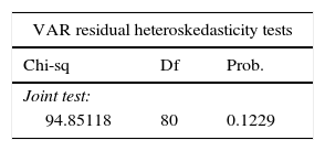
Homoscedasticity

Under the existence of normality in the series of residuals of the unemployment model (median zero and constant variance), we looked to satisfy the assumption that all the terms of error have the same variance, i.e., the errors are homoscedastic (Achen & Shively, 1995).

The proposed unemployment model shows Homoscedasticity in the errors in joint probability (Table 12).

Table 12.

VAR heteroscedasticity test.

VAR residual heteroskedasticity tests
Chi-sq	Df	Prob.
Joint test:
94.85118	80	0.1229

Dependent	R-squared	F(8,53)	Prob.	Chi-sq(8)	Prob.
Individual components:
res1 * res1	0.089999	0.655213	0.7278	5.579946	0.6942
res2 * res2	0.253410	2.248682	0.0379	15.71143	0.0467
res3 * res3	0.085185	0.616901	0.7597	5.281467	0.7271
res4 * res4	0.119979	0.903233	0.5208	7.438727	0.4901
res2 * res1	0.163802	1.297763	0.2649	10.15572	0.2543
res3 * res1	0.283730	2.624309	0.0169	17.59128	0.0245
res3 * res2	0.152236	1.189675	0.3229	9.438631	0.3067
res4 * res1	0.093524	0.683523	0.7039	5.798492	0.6698
res4 * res2	0.118352	0.889340	0.5319	7.337848	0.5007
res4 * res3	0.066492	0.471883	0.8705	4.122475	0.8459

Source: Own elaboration with the use of the econometric analysis package of Eviews8.

Impulse-response functions

The VAR methodology's objective is to isolate primitive sources of economic variability, created by diverse economic, political and social natures, from the public or private sectors, or from the exterior sector of the economy. Therefore, with the VAR modeling there tends to be an interest in the dynamic effects of said primitive disturbances in the evolution of the Unemployment variable that characterizes this study.

In the estimations, the option of generalized impulses posed by Pesaran and Shin (1998) is employed for the estimation of the impulse-response functions. In light of this, the vector function of response to impulse quantifies the effect on the variables of the system, throughout a time horizon, of an isolated impulse equal to the unit in each of the “n” disturbances of the model.

The impulse-response functions help to better visualize the relations between the macroeconomically used variables (Unemployment, Gross Capital Formation, Exports and Monetary Offer). Such functions illustrate the effect that a random shock in one of the variables has on the rest of the variables of the system (Figs. 6–9).

Fig. 6.

Impulse-response function of the unemployment level against a shock in a standard deviation of the same unemployment.

Source: Own elaboration with data obtained from INEGI (2015) and to the use of the package of econometric analysis of Eviews8, level of confidence to 95%.

Fig. 7.

Impulse-response function of the unemployment level against a shock in a standard deviation of exports.

Source: Own elaboration with data obtained from INEGI (2015) and to the use of the package of econometric analysis of Eviews8, level of confidence to 95%.

Fig. 8.

Impulse-response function of the unemployment level against a shock in a standard deviation of the gross capital formation.

Source: Own elaboration with data obtained from INEGI (2015) and to the use of the package of econometric analysis of Eviews8, level of confidence to 95%.

Fig. 9.

Impulse-response function of the unemployment level against a shock in a standard deviation of the monetary attachment M1.

Source: Own elaboration with data obtained from INEGI (2015) and to the use of the package of econometric analysis of Eviews8, level of confidence to 95%.

In the case of the VAR(p) models, that use stationary variables, from which the impulse-response functions of the system are derived. The VEC models, due to being comprised by non-stationary variables, are not represented in this investigation. It is worth remembering that in stationary processes the responses of the variables in the face of random shocks must fall over time, so that they tend toward zero when t → ∞.

Given that the interest of this paper falls on the variable of the percentage of unemployed, the Figures of response for the DES variable in the face of an impulse (random shock) on the DES, GCF, EX, and M1 variables are shown. Orthogonal response impulses will be used built from an innovation of a standard deviation in the transformed method, and the horizon utilized was of 20 periods. That is, the responses of the DES variable were shown in a horizon of five years subsequent to the shock of each independent variable.

As was to be expected, the strongest response in the percentage of unemployed was obtained for a random shock in the GCF investment variable, i.e., if there is a negative shock in investment, its effect is a direct rise on unemployment, which will then have its effect for up to a year, reaching a balance after two and a half years. On the other hand, a labor offer shock has the effect of reducing the percentage of unemployment for up to a year and a half after the initial impulse.

In the sense of an open economy, a shock in exports reduces the percentage of unemployment up to a year following the initial shock; afterwards, the effect turns out to be greater than the initial point, when there is once more an increase in the percentage of unemployment as consequence of stationary behavior since 2010, subsequent to the global liquidity financial crisis. Although the control exerted on the monetary offer has the purpose of controlling the economic effects caused by inflation, this variable shows a direct relation, i.e., in light of a shock in the M1 monetary aggregate; the effect on the percentage of unemployment always results positive throughout the subsequent time horizon. That is, the shock in the M1 causes an increase in unemployment, given that the disposition of liquidity causes a greater demand of goods and services, which is reflected in the productive sector through the increase in its production costs, therefore, said sector is more productive with an increase in gross capital formation and possible reductions in the variable costs of direct labor.

Finally, this investigation gives rise to the identification of possible theoretical non-compliances in future investigations, such as the case of the Phillips Curve law, which in some periods is not applicable as indicated by the methodological origin.

Conclusions

Having highlighted that in Mexico there has been a difficulty in the Unemployment variable to adjust to the levels observed prior to the global financial crisis of 2008, this reflects less labor stability for the Mexican society in the long-term. Therefore, economically determining the hysteresis of Unemployment in Mexico as the long-term impact that persists in said series due to an endogenous shock of its very own historic as that of other macroeconomic variables, i.e., a deviation due to some economic-structural change (Trejo & Vengas, 2010), the determinants of the level of unemployment in Mexico were thus analyzed, with a UVAR model, according to the lack of applicability of a co-integration model (VEC).

The variables used were the Unemployment Rate (DES), the Basic Monetary Aggregate (M1), the Gross Capital Formation (GCF), and the level of Exports (EX). Thus, it was detected that the unemployment rate from 1999 to 2014 has had an upward behavior, with a breakage of 6.15% in 2009 due to the global liquidity crisis. The reason for it is the limited economic activity in Mexico, with yearly economic growths below 3% after the last global crisis and with it a labor reform implemented in the current presidential administration. This coincides with the GCF, a variable with an average quarterly growth of only 2.81% since 2010 until the closure of 2014, showing the low dynamism and the limited economic growth in Mexico. Furthermore, the international environment cannot be overlooked given that as long as the oil prices do not recover and the structural reform of the power sector is not grounded and translated to greater levels of investment in the sector, they will continue to reflect less petroleum exports. Even the monetary policies link their policies in the establishment of inflation, but this has effects on unemployment. The monetary policies link these variables to the quantity of money or interest rate, thus indirectly affecting unemployment.

The presence of hysteresis for unemployment in Mexico was proven, as determined through unitary roots, which indicates that the unemployment model is determined by its history and macroeconomic factors. The shocks of the endogenous M1 and GCF variables are the ones that have a greater and more direct impact on the Unemployment rate in Mexico. In this sense, a large part of the effects of unemployment derive from the liquidity levels of the economy, influenced by the interest rates. Whereas the degree of investment in Mexico continues to be an important factor in the employment of labor, which can be seen reflected in the unemployment level as well as in the increase of exports.

Other exogenous causes of hysteresis to the unemployment model proposed in Mexico, could be due to the depreciation of human capital and the lack of employment possibilities, situation which opens the doors for future investigations. Furthermore, the difference of criteria to account for the groups of unemployed people becomes a factor of much importance, given that disparities were found; one of them is the comparison with the unemployment rates of industrialized countries that are greater than those in Mexico, likewise, the data provided by some of the main institutions is not homogeneous.

Empirical investigations were referenced in this paper regarding the hysteresis of unemployment, in which it was observed that the level of unemployment maintains some tendency in periods subsequent to shocks caused by the economic policy or other random factors. From here the idea that unemployment and the economic activity could evolve in the same direction can be suggested, if the participation rate is pro-cyclical as it happens to be in various periods. It is worth noting that this analysis was carried out in a global manner for the Mexican labor market, and thus a proposal for future investigations to evaluate the economic policies could derive from a demographic framework in order to point out the States that have smaller unemployment persistence rates.