Complex stylized facts of the Mexican economy: a hirschmanian perspective (to attack the “fear of growing”, more and better)

Abstract

We elaborate some complex stylized facts related to the Mexican economy. The analyzed period runs from 1960 to 2013 with selected subperiods. Our main findings are: 1) there are involuntary idle capacities in the manufacturing industries; 2) the growth of the Mexican economy is not balanced but unbalanced; 3) there is an inflation-free environment. This fact is consistent with the previous ones; 4) there is a mixed of efficient and inefficient sequences of investment; 5) the stimulus of manufacturing exports on macroeconomic performance has been offset by its imports; 6) the deficits in manufacturing balance and in the current account have been financed without difficulty. Of course, this financing capacity constitutes a second best condition; 7) according to a backward linkages analysis, the towing capacity of manufacturing sector over the Mexican economy would be a larger one if the manufacturing imports penetration had not been so intense since the trade liberalization; and 8) the size of the positive effect of the manufacturing sector on the economy and on the non-manufacturing sectors diminished since the early eighties. Our complex stylized facts highlight the need for an upgrading of the current economic policies.

Resumen

Elaboramos algunos hechos estilizados complejos relacionados con la economía mexicana. El período analizado se extiende desde 1960 hasta 2013, con subperiodos seleccionados. Nuestras principales conclusiones son las siguientes: 1) existen capacidades ociosas involuntarias en las industrias manufactureras; 2) el crecimiento de la economía mexicana no es balanceado sino desbalanceado; 3) existe un entorno macroeconómico libre de inflación. Este hecho es coherente con los anteriores; 4) se observa una secuencia de inversiones eficientes e ineficientes; 5) el estímulo de las exportaciones manufactureras hacia la economía en su conjunto ha sido parcialmente anulado por sus importaciones; 6) los déficits en la balanza manufacturera y en la cuenta corriente se han financiado sin dificultad. Sobra decir que esta capacidad de financiamiento constituye una segunda mejor opción; 7) de acuerdo con un análisis de encadenamientos hacia atrás, la capacidad de arrastre del sector manufacturero hacia la economía sería mayor si la penetración de las importaciones no hubiera sido tan intensa desde la liberalización del comercio; y 8) el efecto positivo del sector manufacturero en la economía y en los sectores no manufactureros ha disminuido desde principios de los años ochenta. Los hechos propuestos revelan la necesidad de mejorar las políticas económicas aplicadas actualmente.

Introduction

“It is useful from time to time to revisit the pioneers in a field. The richness of their original thought is often diminished as new specialists in a field are educated or, rather, trained. Stylized caricatures and toy models out-compete nuanced multidisciplinary narratives in the competition for shelf-space in textbooks. After the students ingest the textbooks and go forth in the discipline as properly trained specialists, they are hard put just to keep up with the latest publications and to do their own bit to push the frontier forward. Outside of those inclined to intellectual history, the specialists have little occasion to go back to revisit the pioneers.” David Ellerman (2004:311)

Extending the seminal idea proposed by Kaldor (1961), we elaborate some complex stylized facts related to the Mexican economy. The analyzed period runs from 1960 to 2013 with selected subperiods. By the way, the word complex merely recognizes the fact that the functioning of an economy in a globalized world full of innovations and in a heterogeneous society as the Mexican is a challenge that economic policy makers and the private sector have to face in order to accomplish their goals.^a We hope that our complex stylized facts express to some extent these circumstances.^b

Although the stylized facts gathered by Kaldor allegedly sought to be theoretically neutral, our complex stylized facts are inspired in a book, among others, entitled The Strategy of Economic Development written by Albert O. Hirschman (1915-2012) long ago. Other sources of inspiration are Keynes (1936), Kalecki (López & Assous, 2010), Steindl (1976), and Kaldor (1966 and 1967).

Our complex stylized facts tackle relevant characteristics of the Mexican economy. Among others, we analyze some properties of its macroeconomic stability in terms of the convergence of the actual output to its potential, and in terms of the balanced or unbalanced growth of the economy as a whole and its parts. Thereon, the availability of involuntary idle productive capacity in the nineties and in the first decades of this century, and the unbalanced growth all through the analyzed period, are complex stylized facts of the Mexican economy. In the present, both facts are advantages. Some examples are the following.

First example, from a microeconomic perspective a significant margin of spare capacity within companies implies that, in a case of increased demand, firms would be able to increase production without pushing its costs, meaning that the economy could grow faster without generating inflationary pressure. Second, from a macroeconomic perspective under a condition of not complete use of physical capital, a responsible deficit is not a risk to macroeconomic stability. On the contrary, represents a policy instrument to narrow the gap between both economic activity levels, which by the way would generate positive effects in the short term and long term, among others a boost in investment. Third example, to move from an economy with certain characteristics to another superior one, the current productive structure has to be altered.

The existence of an inflation-free environment constitutes another complex stylized fact of the Mexican economy. This fact is consistent with the previous ones. Some of the evidence is the following. By no means the variations in prices are neither widespread nor sustained in the Mexican economy between 2008 and 2013. It seems that the positive and negative variations in prices obey to rather idiosyncratic conditions by producer sector, instead of responding to a generalized situation determine by a presumable disequilibrium between aggregated supply and demand, or by an outstanding macroeconomic performance.

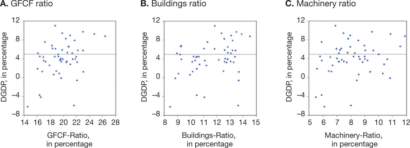
The mixed of efficient and inefficient sequences of investment constitute another complex stylized fact of the Mexican economy. Therefore, it seems feasible to reach an adequate economic growth rate without the need to substantially increase the investment ratios, or equivalently, the internal and external funding. Some of the facts are the following. First, it is patent the relationship between investment ratios (GFCF/GDP for example) and economic growth all through the analyzed period. Second, the range of investment ratios is particularly narrow, considering the wide range of economic growth rates. Historically speaking, an economic growth rate proximate to 5 is linked with numerous investment ratios. Third, there is not a consistent match between the values of the ratios and the economic growth rates if we order all them from highest to lowest. And fourth, the macroeconomic returns of the investment efforts are not the same during the analyzed period, that is to say, there is a diminishing impact of investment on economic growth.

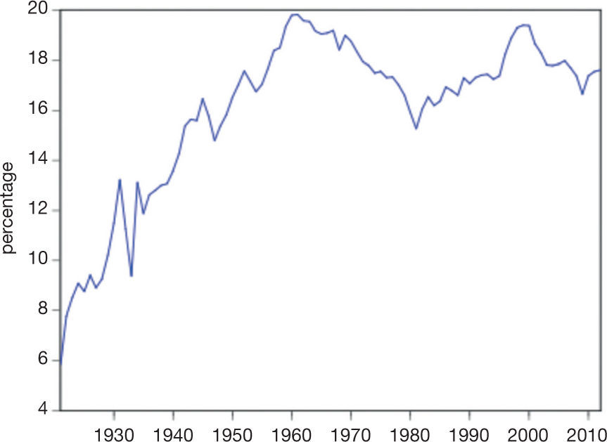
From 1960 to 2012 the share of the manufacturing as a percentage of the GDP ranged slightly from 15% to 20%. In the 60's and 70's, there is a trend with a negative slope in the share, but since 1981 there is a positive one. Even so, the size of the positive effect of the manufacturing sector on the economy and the non-manufacturing sectors, that is the elasticity, has diminished during the analyzed period. The above constitutes another complex stylized fact of the Mexican economy. To support our claim, we analyze the external balance of manufacturing with a slightly global value chains emphasis, and its backward linkages using three official input-output matrices.

Before starting, we want to explicit our intentions. Bearing in mind Kaldor (1961), we hope that our complex stylized facts serve to the economist community to agree on the main features of the Mexican economy. Of course, the next step would be its joint explanation. As will be justified in the final reflections, our complex stylized facts highlight the need for an upgrading of the current economic policies. In this sense, to attack the “fear of growing” more and better, that suffer the economic policy makers in Mexico, among many others countries, one of the mantras proposed reads as follows, “grow, grow and grow”.^c

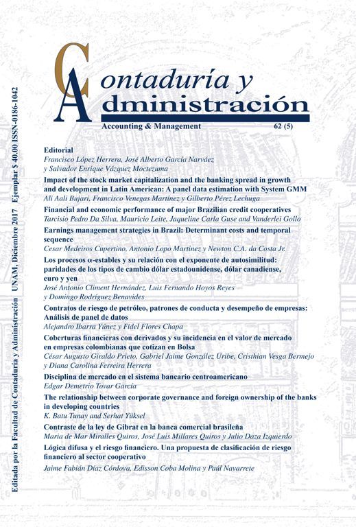
Actual and potential output

An outstanding characteristic of the Mexican economy is its macroeconomic stability. Basically, it is the result of economic policies and institutional reforms that have been implemented since the debt crisis at the beginning of the eighties. In this sense, the transformation of the Mexican economy should be understood as a nonstop process. Among the alternatives to illustrate this feature, a favorite one has been to establish the convergence of the actual output to its potential (see for example Carstens, 2013b:10), using a smoothing tool known as Hodrick-Prescott filter.^d The presumption of a balanced growth, as appears in Fig 1, is a consequence of this tradition.

Fig. 1.

Actual and potential output, 1993-2013, monthly data.

Source: own calculations using data from the National Accounts System, INEGI.

The reference to the Hodrick-Prescott filter and other ones, with and without corrections, is a common place in the applied literature. In an attempt to avoid the boundaries of the HP filter and of the modeling of a production function, in the so-called Criterios Generales de Política Económica 2014 (Presidencia de la República, 2013:76) the potential output was established as an average of economic growth rates registered during a “relatively long period”. However, following the same tradition of the contemporary macroeconomics, according to this “simple and transparent” exercise of smoothing, the economy regularly operates under complete use of its physical capital.

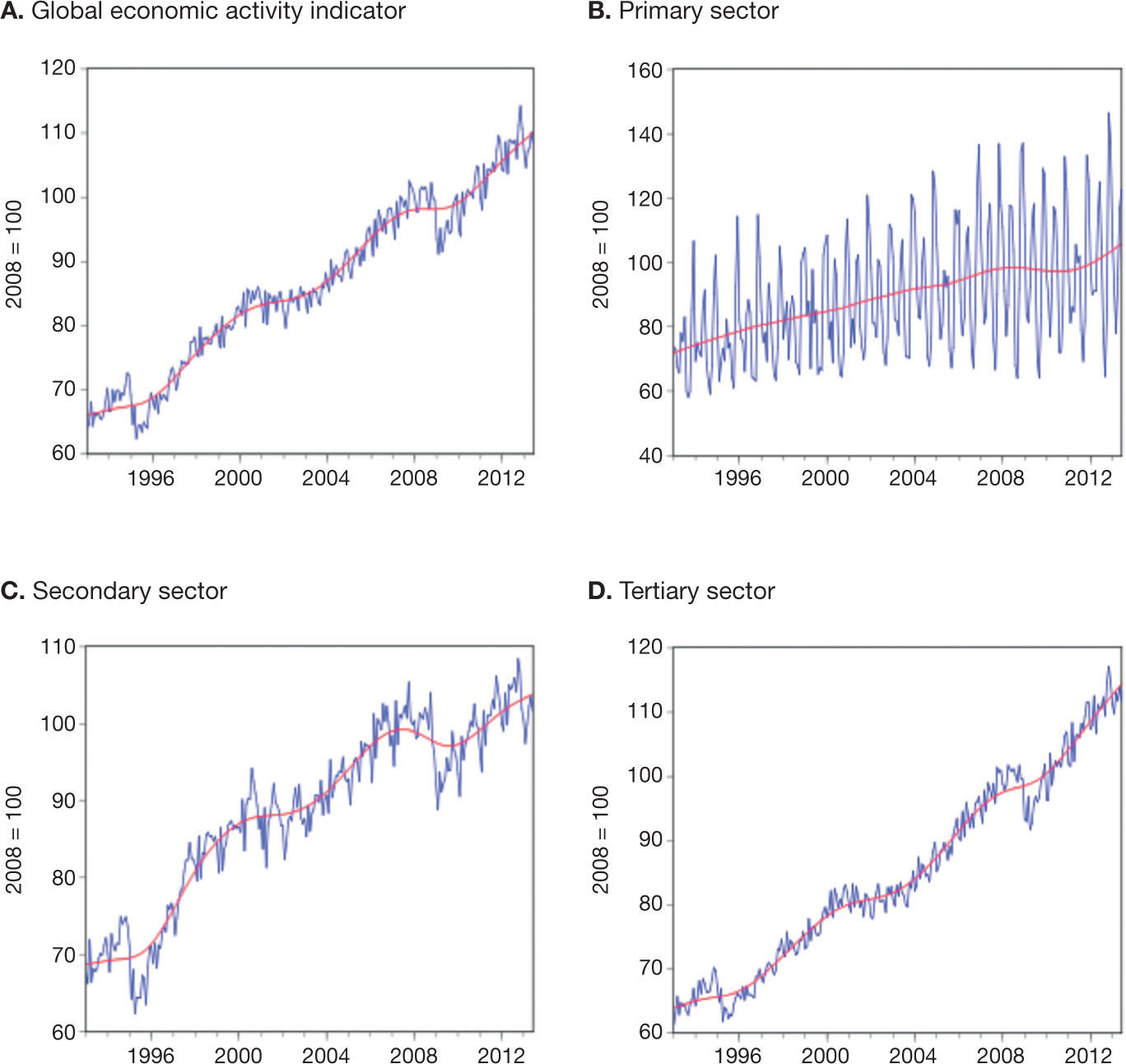
If we use the same mathematical definition of potential output into a broader period, then we could easily establish the same characteristic of the Mexican economy as appears in the next figure (Fig. 2).

Fig. 2.

Actual and potential output, 1929-2012, annual data.

Source: own calculations using data from the National Accounts System, INEGI.

A visible limit of this tradition is that the potential output, theoretically defined as the output level associated with the efficient and full employment of productive resources in an economy, is a non-observable variable, which means that its measurement, being optimistically, is full of obstacles.^e It is worthwhile to remark that the quantification of physical capital and labor into a single economic unit is a difficult task. Suffice to say that systematically economic units do not value its physical capital correctly, and there is a severe deficiency in terms of aggregate volume measurements cause by the unavailability of individual price indexes and by the not fully quality adjustment of the aggregate ones (Guerrero, 2009 and 2013).^f By the way, the evolution of hours worked in time is another challenge in terms of its quality adjustment.^g

The hearth of the matter is that the statement about the convergence of the actual GDP to its potential is rather theoretical, specifically it constitutes an assumption, and by the way a distinguishing one.^h Therefore, we think it is a debatable position. In first place, there is not a correspondence between the theoretical definition and its practical measurement. In second place, from an alternative tradition it has been argued that market economies do not generate, automatically, enough aggregate demand in order to match actual and potential output. In this sense, the equalization of the levels of economic activity is a rare episode, and there are not repeated sequences of recessionary gaps and inflationary gaps as are conceptualized by this tradition. There is only one aggregated supply curve, which does not distinguish the short term and the long term, with a vertical portion at the end of it.

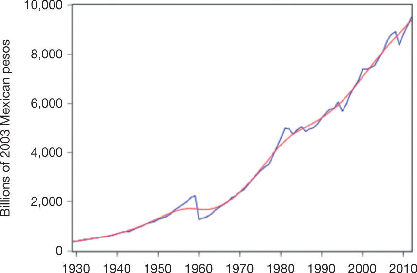
The degree of use of installed capacity is a key variable in order to evaluate the magnitude of the convergence of actual output to its potential, and to understand the investment decisions (Steindl, 1952).ⁱ The following scatter plot shows the degree of use as a percentage and the growth rate of real output in manufacturing, between 1994 and 2013 (Fig. 3).

Fig. 3.

Degree of use of installed capacity and growth rate of real output in manufacturing, 1994-2013, monthly data.

Source: own calculations using data from Monthly Surveys of Manufacturing Industries, CMAP and EMIM, INEGI.

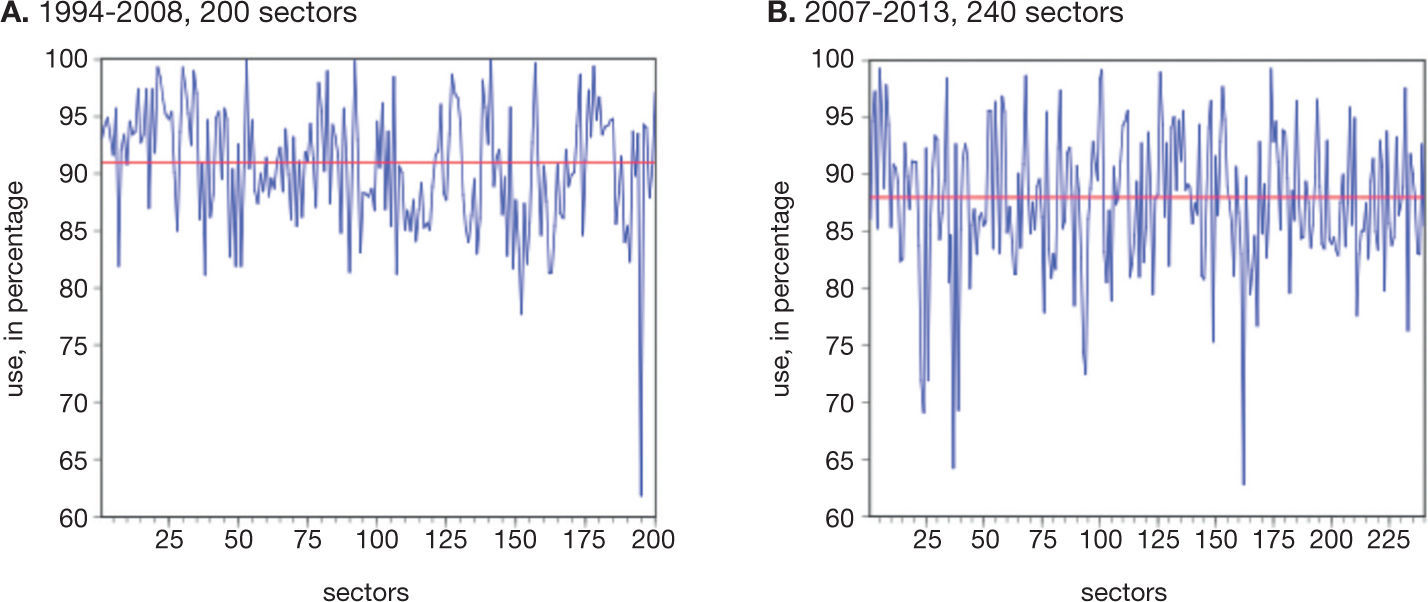
As expected, there is a positive relationship between growth rate of real output and the percentage of use of installed capacity. Throughout the analyzed period, the range of use of physical capital in the manufacturing was between 74 and 86 percent. It is fascinating and invites speculation to note that, in the first panel, a range between 80 and 82 of use of physical capital is linked with a cloud of growth rates that range from –5% to 18%, by the way the maximum value during the analyzed period. Something similar can be said about the second panel. Regardless of the month and year, the Figure 4 shows the maximum values of the degree of use of installed capacity reported by sector.

Fig. 4.

Maximum degree of use of installed capacity, manufacturing sectors, 1994-2013, monthly data.

Source: own calculations using data from Monthly Surveys of Manufacturing Industries, CMAP and EMIM INEGI.

All through the analyzed period, it seems that there are involuntary idle capacities in both, individual activities and in the manufacturing as a whole. The above constitutes a complex stylized fact of the Mexican economy, which is opposed to the previous tradition that determines potential output by means of a growth component. In the same direction, using a Kaleckian background, Guerrero (2012) estimated that if the manufacturing sectors had fully utilized its production capacity between 2003 and 2008, the average rate of growth of the Mexican economy would have been 6.81% and not 3.36%. As is well known two caveats to our interpretation are the following. The first one, the idle capacity, technically speaking, is necessary. The second one, the idle capacity may not be competitive at the time by market conditions. Although the gap between growth rates proposed by Guerrero (2012) may sound excessive, it simply constitutes a reference point regarding the latent capabilities of the Mexican economy in the short run.

As was noted at the beginning of this section, one implication of the first perspective revised is that the dynamic of the economy is a balanced one, whatever that means. Nonetheless, according to Hirschman (1959:51-2) the favourable case is the unbalanced path in the following context^j:

“In this version the requirement of balanced growth is derived from the demand side. It is argued that a new venture –say, a shoe factory– which gets underway by itself in an underdeveloped country is likely to turn into a failure: the workers, employees, and owners of the shoe factory will obviously not buy all its output, while the other citizens of the country are caught in an “underdevelopment equilibrium” where they are just able jointly to afford their own meager output. Therefore, it is argued, to make development possible it is necessary to start, at one and the same time, a large number of new industries which will be each others’ clients through the purchases of their workers, employees, and owners. For this reason, the theory has now been annexed to the ‘theory of the big push’. A big push could, of course, result from one or a few big projects, or from a large number of projects of varying size that dovetail with one another. It is clearly the latter alternative of the ‘big push’ theory that is implied by the theory of balanced growth… My principal point is that the theory fails as a theory of development. Development presumably means the process of change of one type of economy into some other more advanced type. But such a process is given up as hopeless by the balanced growth theory which finds it difficult to visualize how the ‘underdevelopment equilibrium’ can be broken into at any one point.”

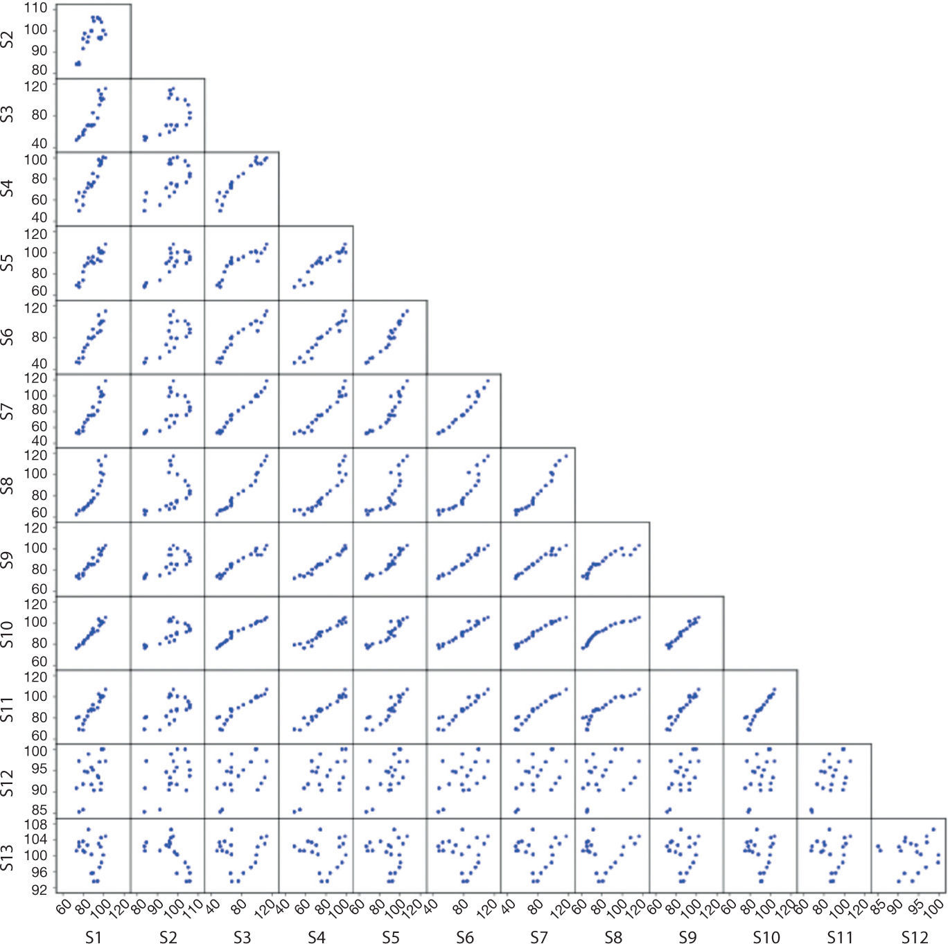
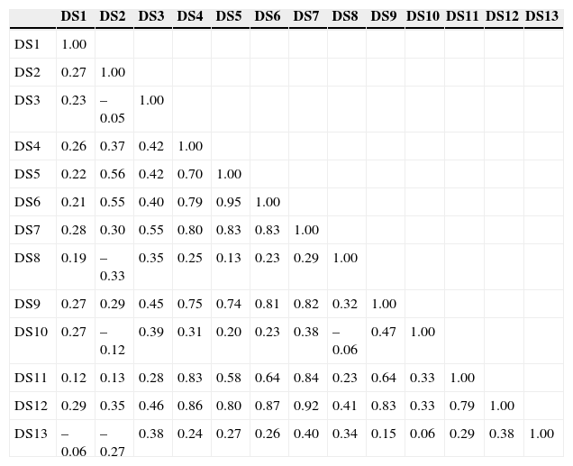
As a first step to explore the unbalanced hypothesis, the following scatter plot shows the Mexican economy disaggregated by thirteen sectors from 1993 to 2012 with annual frequency (Fig. 5).^k

Fig. 5.

Mexican economy disaggregated by thirteen sectors, in levels (2008=100), 1993-2012, annual data.

Source: own calculations using data from the National Accounts System, INEGI.

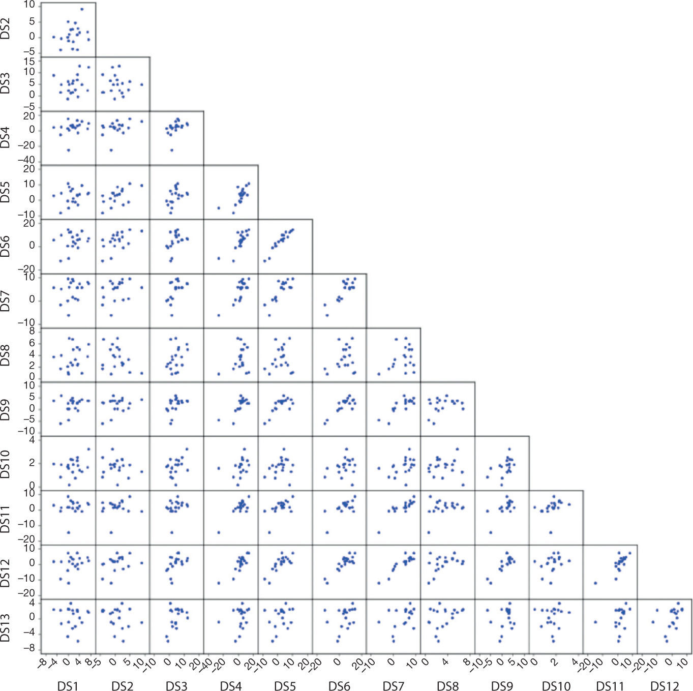
Broadly speaking, there are co-movements between the levels of economic activity by sectors, more clearly in some cases than in others. In the case of sectors 12 and 13, that is, “Accommodation and food services”, and “Legislative, justice, etc.” definitely that is not the case. The figure allows us to find out some nonlinear relationships between the analyzed variables (Fig. 6). The next scatter-plot shows the variables in growth rates.

Fig. 6.

Growth rates in percentage, thirteen sectors, 1994-2012, annual data.

Source: own calculations using data from the National Accounts System, INEGI.

It seems that the balanced growth hypothesis is not supported by the information content in the figures; in other words, there is evidence in favor of the Hirschmanian hypothesis in the case of the Mexican economy during the analyzed period.

We want to close this section with two observations. The first one, the determination of potential output in an economy strongly linked with the rest of the world should be upgraded in the sense of taking into account not only the domestic productive resources but also, to some extent, the external ones. In order to measure this broad definition of potential output, one concept that should be explicit is the so-called sustainable imports level. The second one, the hypothesis about the balanced or unbalanced growth in a globalized economy is a subordinated one. The heart of the matter is rather if the economies have, for example, a sustainable current account. Later we will continue analyzing this concern.

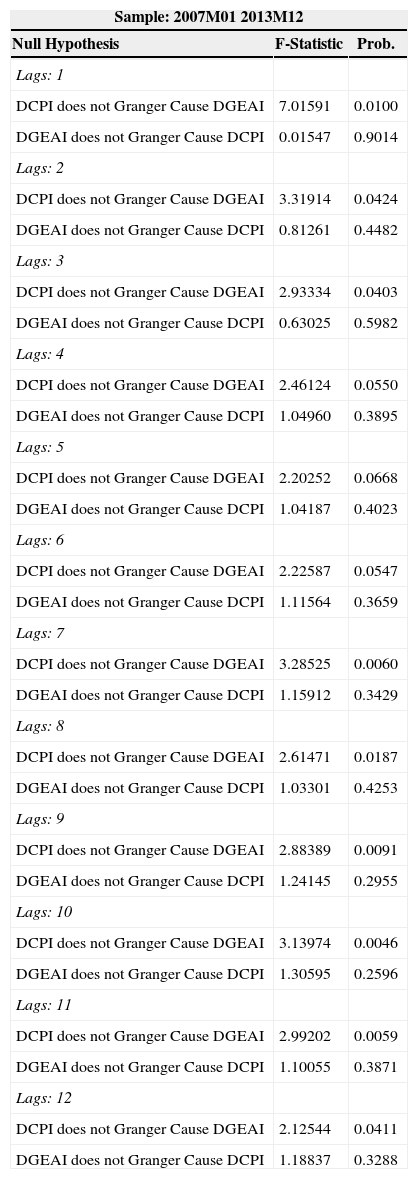
Inflation

Inflation is a summary measure of variations in prices of goods and services consumed by households. From an aggregate point of view, to some extent, it reveals the disequilibrium between aggregated supply and demand. In this sense, in the Appendix we show the results of Granger causality tests from one lag to twelve (monthly data) between 2008 and 2013. In all cases, the causality runs exclusively from the economic growth rate to inflation –that makes sense.

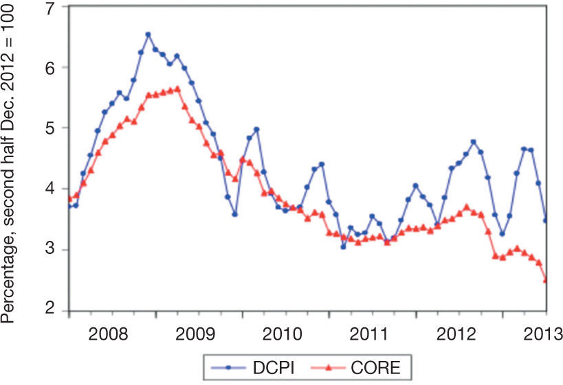
According to an orthodox macroeconomic point of view, inflation refers, strictly, to the widespread and sustained increase in prices over time. Based on the Mexican consumer price index, the following figure (Fig. 7) shows the general inflation and the core one. The starting point was selected considering the current monetary policy framework.

Fig. 7.

General and core inflation, 2008-2013, monthly data.

Source: own calculations using data from INEGI.

Let us begin with a truism, the negative slopes point out that there is not a sustained increase in prices over time, at least in the analyzed period. Among other factors, the competitive environment created by the open economy has played a positive role. Certainly, the inflation-targeting regime has been effective as a nominal anchor of the economy. Since then, the set of actions taken by the Mexican Central Bank has been, evidently, one key of the success. Its handling of expectation, for example, has been formidable. The question of the role played by the nominal exchange rate, or other nominal price, for example the minimum wage, exceeds the purpose of this document.

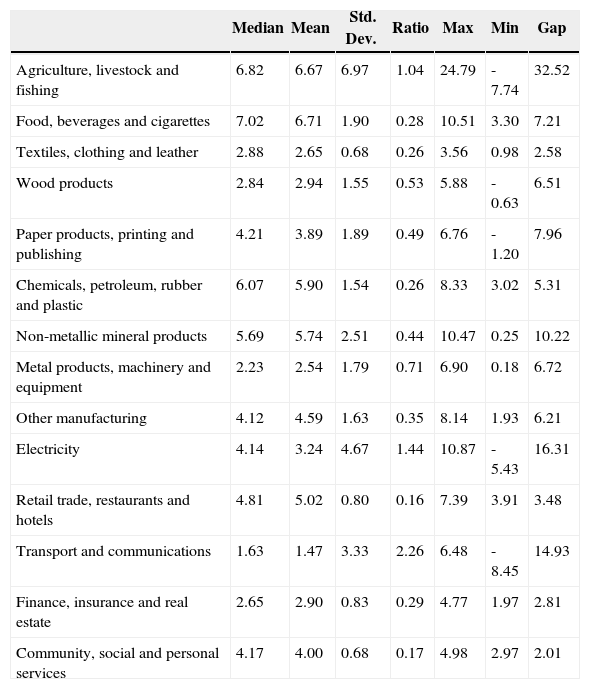
The following table (Table 1) shows statistics by every one of the producer sector of the goods and services included in the CPI. As the gentle reader will notice, the disaggregated analysis will help us to understand differently the relationship between the dynamics of prices and economic activities.

Table 1.

Growth rate of CPI components by producer sector, 2008-2013, monthly data.

	Median	Mean	Std. Dev.	Ratio	Max	Min	Gap
Agriculture, livestock and fishing	6.82	6.67	6.97	1.04	24.79	-7.74	32.52
Food, beverages and cigarettes	7.02	6.71	1.90	0.28	10.51	3.30	7.21
Textiles, clothing and leather	2.88	2.65	0.68	0.26	3.56	0.98	2.58
Wood products	2.84	2.94	1.55	0.53	5.88	-0.63	6.51
Paper products, printing and publishing	4.21	3.89	1.89	0.49	6.76	-1.20	7.96
Chemicals, petroleum, rubber and plastic	6.07	5.90	1.54	0.26	8.33	3.02	5.31
Non-metallic mineral products	5.69	5.74	2.51	0.44	10.47	0.25	10.22
Metal products, machinery and equipment	2.23	2.54	1.79	0.71	6.90	0.18	6.72
Other manufacturing	4.12	4.59	1.63	0.35	8.14	1.93	6.21
Electricity	4.14	3.24	4.67	1.44	10.87	-5.43	16.31
Retail trade, restaurants and hotels	4.81	5.02	0.80	0.16	7.39	3.91	3.48
Transport and communications	1.63	1.47	3.33	2.26	6.48	-8.45	14.93
Finance, insurance and real estate	2.65	2.90	0.83	0.29	4.77	1.97	2.81
Community, social and personal services	4.17	4.00	0.68	0.17	4.98	2.97	2.01

Source: own calculations using data from INEGI.

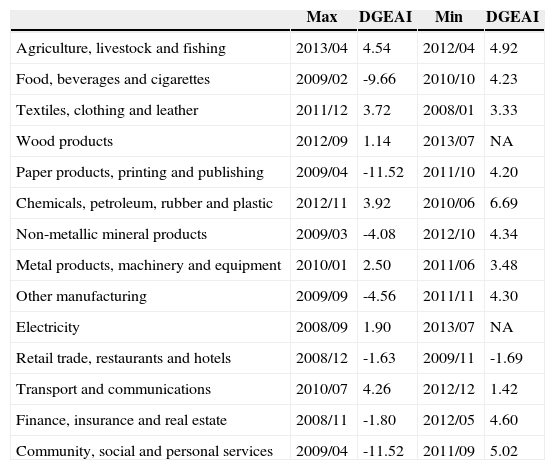
It is worth emphasizing at least the following. First, if we compare medians or means, or maximum and minimum values, or gaps, or ratios calculated using means and standard deviations, between sectors, there is not an indiscriminate increase in prices during the analyzed period. Just a few examples. Five of the 14 sectors reported inflation lower than 3%. Only three sectors shown variability in terms of its ratio, that is to say, greater than one. And the difference between maximum and minimum values show quite heterogeneity in terms of the response between sectors, that evidently share the same general condition of the economy. The following table (Table 2) shows the maximum and minimum by date, and its corresponding observed economic growth rate based on the Global Economic Activity Indicator.

Table 2.

Growth rate of CPI components by producer sector, and economic growth rate, 2008-2013, monthly data.

	Max	DGEAI	Min	DGEAI
Agriculture, livestock and fishing	2013/04	4.54	2012/04	4.92
Food, beverages and cigarettes	2009/02	-9.66	2010/10	4.23
Textiles, clothing and leather	2011/12	3.72	2008/01	3.33
Wood products	2012/09	1.14	2013/07	NA
Paper products, printing and publishing	2009/04	-11.52	2011/10	4.20
Chemicals, petroleum, rubber and plastic	2012/11	3.92	2010/06	6.69
Non-metallic mineral products	2009/03	-4.08	2012/10	4.34
Metal products, machinery and equipment	2010/01	2.50	2011/06	3.48
Other manufacturing	2009/09	-4.56	2011/11	4.30
Electricity	2008/09	1.90	2013/07	NA
Retail trade, restaurants and hotels	2008/12	-1.63	2009/11	-1.69
Transport and communications	2010/07	4.26	2012/12	1.42
Finance, insurance and real estate	2008/11	-1.80	2012/05	4.60
Community, social and personal services	2009/04	-11.52	2011/09	5.02

Source: own calculations using data from INEGI.

The extreme values do not shared dates, not even in the case of maximum values, much less in the case of minimums; and there are maximum values in condition of negative economic growth rates, and vice versa! As a matter of fact only in the case of one minimum value, related to “Retail trade, restaurants and hotels”, the observed growth rate of the Global Economic Activity Indicator was negative.

By no means variations in prices are neither widespread nor sustained in the Mexican economy from 2008 to date. It seems that the positive and negative variations in prices obey to rather idiosyncratic conditions by producer sector, instead of responding to a generalized situation determine by a presumable disequilibrium between aggregated supply and demand, or by an outstanding macroeconomic performance –what indeed constitutes a ruthless tale if we remember that between 2008 and 2013 the Mexican economy grew at an average annual rate of 1.84%, pretty far from its potential growth rate figure. Therefore, the existence of an inflation-free environment constitutes a complex stylized fact of the Mexican economy.

Last but not least, another argument, which goes beyond the purposes of this document, is linked with the fact that, frequently, official prices indexes do not completely adjust for changes in quality (Guerrero, 2008a). Notably, disregarding improves in quality leads to an overstatement of price changes and to an underestimation of economic growth (Guerrero, 2008b; Schreyer, 1996 and 1998).

We want to end this section noting the following. In first place, it is better to make a distinction between the theoretical definition of inflation and its measurement, inspired by the Mexican Central Bank's objective. In this sense, arithmetically speaking, a positive variation in the consumer price index is called inflation, and ceteris paribus, it affects the stability of the domestic currency's purchasing power, or put it correctly, the purchasing power of people.

In second place, in essence the inflation reflects always and everywhere a distributional conflict. In modern words, inflation reflects the dispute over the value added by economic agents, internal and external, which becomes visible by means of variations of nominal prices, that is, profits, wages, taxes, and the exchange rate. The most feared situation, when a government runs a deficit financed by printing money or financed with tax increases, all that is manifesting is a bargain to increase its share in the value added, at the expense of other players. From this perspective, the Mexican Central Bank's real success has been the containment of the dispute between the agents. Certainly, self-restraint of the claims of economic agents has contributed to generate an inflation-free environment.

In third place, inflation constitutes a permanent risk for economies, which simply reveals the insistence of agents with market power to increase their slice of the pie. Policy makers should combat attempts of this kind of abuse.

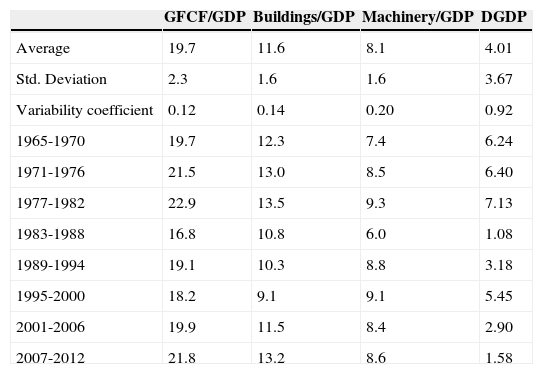
Investment

The investment determines what is produced and, to some extent, what is exported. According to Albert O. Hirschman, the “investment choices” constitutes the crucial problem in the development theory and policy, and the problem in our economies is, precisely, the shortage of “ability to invest”. It is interesting to note that, for our guru, the issue relating to the funding of investment is, relatively, secondary. We show some investment ratios and economic growth rates next (Fig. 8; emsp Table 3).

Fig. 8.

Investment ratios as a percentage of GDP and growth rates of GDP, 1960-2012, annual data.

Source: own calculations using data from the National Accounts System, INEGI.

Table 3.

Investment ratios and growth rates of GDP, 1960-2012.

	GFCF/GDP	Buildings/GDP	Machinery/GDP	DGDP
Average	19.7	11.6	8.1	4.01
Std. Deviation	2.3	1.6	1.6	3.67
Variability coefficient	0.12	0.14	0.20	0.92
1965-1970	19.7	12.3	7.4	6.24
1971-1976	21.5	13.0	8.5	6.40
1977-1982	22.9	13.5	9.3	7.13
1983-1988	16.8	10.8	6.0	1.08
1989-1994	19.1	10.3	8.8	3.18
1995-2000	18.2	9.1	9.1	5.45
2001-2006	19.9	11.5	8.4	2.90
2007-2012	21.8	13.2	8.6	1.58

Source: own calculations using data from the National Accounts System, INEGI.

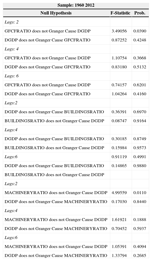
One interpretation of the above statistical information is the following. In first place, it is patent the association between investment ratios and economic growth in averages. To complement this, in the Appendix we show the results of Granger causality test between the investment ratios and the economic growth. As expected, according to this statistical exercise the causality runs in both directions, from ratios to growth and vice versa. In second, the range of investment ratios is particularly narrow, considering the wide range of economic growth rates. As is shown in the Figure 8 an economic growth rate proximate to 5 is linked with numerous investment ratios. In third, there is not a consistent match between the values of the ratios and the economic average growth rates if we order all them from highest to lowest. The two worst examples are the following. In 2007-2012 the investment ratios were highest than the ones reported in 2001-2006, but the economic growth rate was almost the double in 2001-2006 with respect to 2007-2012. From the hand of the second highest GFCF/GDP ratio, the economic growth rate ranked the second last place during 2007-2012, just above the worst rate registered in 1983-1988. In fourth place, the macroeconomic returns of the investment efforts are not the same during the analyzed period, that is to say, there is a diminishing impact of investment on economic growth.

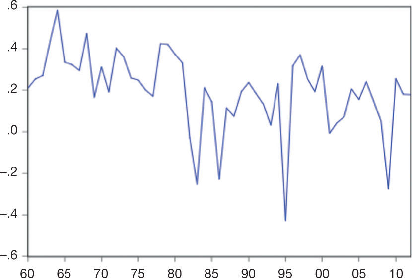
As a mechanism to further explore our hypotheses derived from the contents of the above figure and table, we applied a time varying approximation with the purpose of examine the changing effect of the Gross Fixed Capital Formation (GFCF) ratio on the economy growth rate. In the observation equation (1) the elasticity is specified as a time-varying coefficient, and in the state equation (2) as a first order autoregressive process:

The system of equations were estimated using a forecast recursive algorithm known as Kalman filter. The next figure shows our statistical results (Fig. 9).

Fig. 9.

Impact of the GFCF ratio on the economic growth rate, 1960-2012.

Source: own calculations using data from the National Accounts System, INEGI.

The contents of the graph suggests that the impact of the Gross Fixed Capital Formation ratio on the rate of economic growth is changing in time, in some years is positive and in others is negative, the elasticity range is wide, from 0.6 to –0.5, and that its trend is slightly negative. In short, it seems that the mixed of efficient and inefficient sequences of investments constitute a complex stylized fact of the Mexican economy. Being optimistic, it constitutes an opportunity because it seems feasible to reach an adequate economic growth rate without the need to substantially increase the investment ratios, or equivalently, the internal and external funding. Again, this statement is also opposed to Shiau, Kilpatrick, and Matthews (2002), among many others.

About the role of manufacturing in the Mexican economy

According to Kaldor (1966 and 1967) manufacturing has characteristics that make it the engine of economic growth. For dimensioning the size of the manufacturing, the following figure (Fig. 10). depicts its weight as a percentage of the Mexican economy:

Fig. 10.

The manufacturing as a percentage of the overall economy, 1921-2012, annual data.

Source: own calculations using data from the National Accounts System, INEGI.

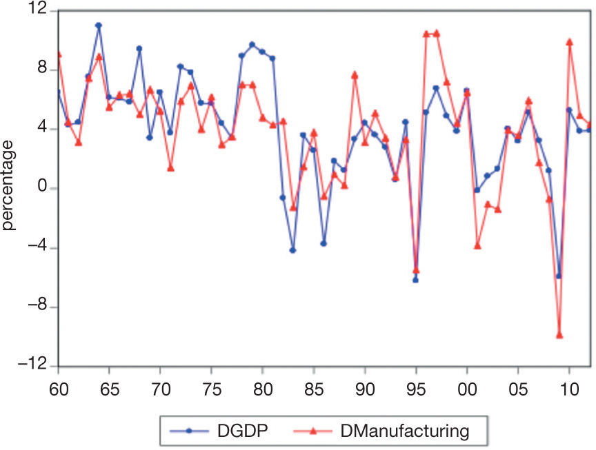
Between 1960 and 2012, the share of the manufacturing in the economy ranged from 15 to 20 percent. By the way, in The Atlas of Economic Complexity (Hausmann et al., 2011), Mexican economy ranked in the number 20, above, among others, Spain (28), China (29), Canada (41), Costa Rica (49), and Brazil (52).^l This remarkable ranking speaks of the outstanding capabilities of the Mexican economy and its manufacturing sector. As another way to illustrate the strong link between the manufacturing and the economy as a whole, the following figure depicts its growth rates (Fig. 11).

Fig. 11.

Growth rates, manufacturing sector and overall economy, 1960-2012, annual data.

Source: own calculations using data from the National Accounts System, INEGI.

We estimated a VAR model in order to analyze the relationship between the manufacturing and the economy as a whole. We use three lags based on lag length tests (see the Appendix). The functional form was the common one, namely, the log-log. We also applied a set of tests to verify the no-autocorrelation, the normality, the no-heteroskedasticity, weak exogeneity, and the stability condition of the VAR. According to Johansen tests (without intercept or trend), there is a long run co-movement between the levels of the variables. The elasticity rose to 1.10.

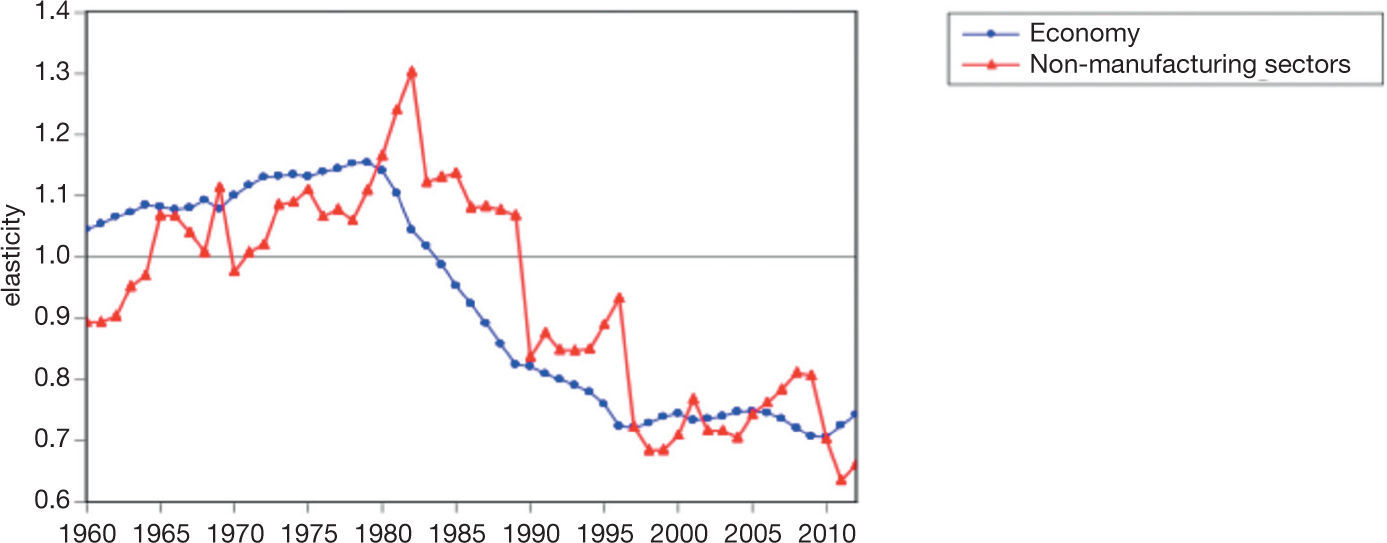
Clearly, the lineal approach is a limited one, so we applied a time varying approximation with the purpose of examine the changing effect of the manufacturing on the overall economy and on the non-manufacturing sectors. In the observation equations (3) and (5), the elasticities are specified as time-varying coefficients, and in the state equation (4) and (6) as first order autoregressive processes:

The systems of equations were estimated using a forecast recursive algorithm known as Kalman filter. The next figure (Fig. 12) shows our results.

Fig. 12.

Impact of the manufacturing on Mexican economy, 1960-2012.

Source: own calculations using data from the National Accounts System, INEGI.

The figure 12 is fascinating and invites speculation. Suffice to say that the size of the positive effect of the manufacturing sector on the economy and on the non-manufacturing sectors has diminished during the analyzed period. The above constitutes another complex stylized fact of the Mexican economy.

Perhaps the reader shares the following questions. How not to think that our proposed stylized fact simply reflects the fact that the growths of manufacturing, of non-manufacturing sectors and of the economy as a whole were different? How to reconcile our proposed stylized fact with the statistical fact according to which the share of the manufacturing in the economy has been relatively stable? Two routes to answer the questions are the following. The first one points to the external balance of manufacturing with a slightly global value chains emphasis, and the second one to the manufacturing backward linkages. We will follow both directions next.

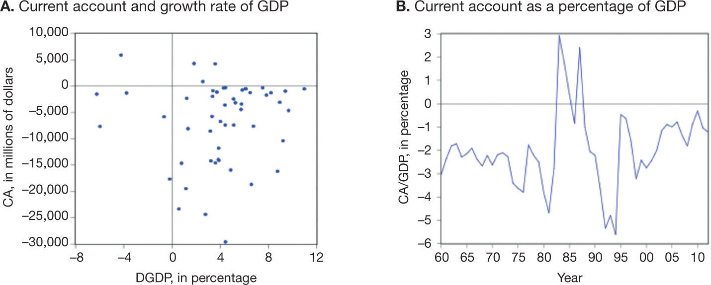
Current account

Bearing in mind an external-constrained growth model, figure 13 shows a scatter plot of the current account and the economic growth rate, and the current account as a percentage of GDP.

Fig. 13.

Current account and growth rate of GDP, millions of dollars and percentage, 1960-2012, annual data.

Source: own calculations using data from the Balanced of Payments, Mexican Central Bank, and the National Accounts System, INEGI.

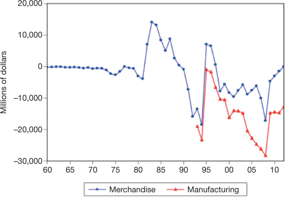
Only from 1983 to 1985 and in 1987, the current account was positive. Most of the points are located in the quadrant corresponding to a deficit in the current account and a positive economic growth rate. Therefore, the current account as a percentage of GDP has been negative in most of the years. Figure 14 shows the merchandise and the manufacturing balances during the analyzed period.

Fig. 14.

Merchandise and manufacturing balances, millions of dollars, 1960-2012, annual data.

Source: own calculations using data from the Balanced of Payments, Mexican Central Bank.

We require two steps in order to formulate a reasonable interpretation of the empirical evidence. First step. From a macroeconomic point of view, it would be better to have a zero balance or a surplus in manufacturing instead of a permanent deficit, in the sense that the stimulus of manufacturing exports flies away to other countries in the form of manufacturing imports. In other words, the stimulus of manufacturing exports on macroeconomic performance and on total employment is offset by the manufacturing imports.^m

The above is useful to explain the diminished impact of the manufacturing sector in the economy.

In terms of the export performance of countries within Global Value Chains, the evidence is the following.ⁿ It is necessary to point out that there are two activities along the value chain, the upstream activities (i.e. the production of intermediate inputs) and more downstream activities (e.g. the final assembly of products). Mexico's integration with the US in regional value chains is a story of contrasts because (OECD, undated:2):

“On average, the foreign value-added content in Mexico's gross exports is larger than in most OECD countries: 32%, compared to the OECD unweighted average of 28%. This is because Mexico is highly involved in international production networks and processing trade. Global value chains are particularly prevalent in electronics, where the foreign content share of more than 60% reflects specialisation in downstream stages of the value chain… and in transport equipment, where over 60% of imported intermediate inputs are destined for export…Services represent a significant share of the value of exports in most manufacturing industries, highlighting the fact that services are more traded than usually thought when taking into account value-added flows… Services account for 6% of gross exports but 31% of exported value-added. However this share of services value-added in exports is the lowest of OECD economies (the OECD unweighted average is 51%) and a third of the services content of exports comes from foreign embodied services, indicating that Mexican firms specialise in manufacturing sectors and in stages of production less intensive in services.”

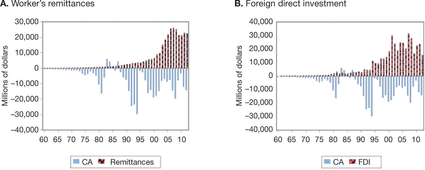
Second step. Despite the deficits, the current account of the balance of payments has been sustainable over time. About financing of the negative balances we want to highlight the role of the worker's remittances and the foreign direct investment, as is shown in the next figure (Fig. 15).

Fig. 15.

Current account and worker's remittances, and foreign direct investment, 1960-2012, annual data.

Source: own calculations using data from the Balanced of Payments, Mexican Central Bank.

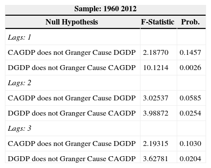
The deficits in manufacturing balance and in the current account have been financed without difficulty by, among others accounts, worker's remittances and foreign direct investment. However, this financing capacity constitutes a second best economic condition. In first place, because much of the macroeconomic stimulus that is originated in exports is lost in imports, with structural effects on the economy as we shall see in the next section. In second place, because it provokes some degree of vulnerability in the sense that the Mexican economy does not fully control, among others, to the foreign direct investment. In the third place, because it may represent a dangerous imbalanced in the case of accelerated economic growth. And in fourth place, because the success of our economy as exporting power or as complex economy is, to some extent, spurious. As a statistical result, the Granger causality tests, that are included in the Appendix, show that the causality runs exclusively from the economic growth rate to the current account ratio –that is consistent with the fact that the performance of the current account depends on the dynamic of the GDP and with the financing capacity of the deficit. All the above constitutes another complex stylized fact of the Mexican economy.

Total backward linkages

For Albert O. Hirschman, the quality of an investment sequence is detectable using as a tool the so-called linkages. A general definition of linkages is the following (Hirschman, 1987:206):

“A linkage (or linkage effect) was originally defined as a characteristic, more or less compelling sequence of investment decisions occurring in the course of industrialization and, more generally, of economic development… The resulting ‘strategy of unbalanced growth’ values investment decisions not only because of their immediate contribution to output, but because of the larger or smaller impulse such decisions are likely to impart to further investment, that is, because of their linkages.”

Specifically, Hirschman (1987:206) explains backward and forward linkages as follows:

“First, an existing industrial operation, relying initially on imports not only for its equipment and machinery, but also for many of its material inputs, would make for pressures towards the domestic manufacture of these inputs and eventually towards a domestic capital goods industry. This dynamic was called backward linkage, since the direction of the stimulus towards further investment flows from the finished article back towards the semi-processed or raw materials from which it is made or towards the machines which help make it… Another stimulus towards additional investment points in the other direction and is therefore called forward linkages: the existence of a given product line A, which is a final demand good or is used as an input in line B, acts as stimulant to the establishment of another line C which can also use A as an input.”

One of the characteristics of the research done by Hirschman (1987:206) was to introduce the economic policy dimension:

“The stimuli towards further investment are rather different for backward and forward linkages. The pressures towards backward linkage investment arise in part from normal entrepreneurial behavior, given the newly available market for intermediate goods. But there may also be resistance against such investments on the part of established industrialists who prefer to continue relying on imported inputs for price and quality reasons. At the same time, state policies favour backward linkage investments (which hold out the promise of foreign exchange savings and of a more ‘integrated’ industrial structure) through the promise of tariff protection and through various preferential foreign exchange and credit allocations, particularly in periods of foreign exchange stringency. The pressures towards forward linkage investment come primarily from the efforts of existing producers to increase and diversify the market for their products. In contrast to backward linkage, there will be only whole-hearted support for backward linkage on the part of existing domestic producers. On the other hand, official development policy is not likely to be particularly concerned with promoting forward linkage investments.”

There are available input-output matrices for the total and internal economy for the years 1993, 2003 and 2008. The difference between total economy and internal economy is that the first distributes the imports among the sectors in the intermediate demand matrix, or in other words, that the second one does not includes imports.

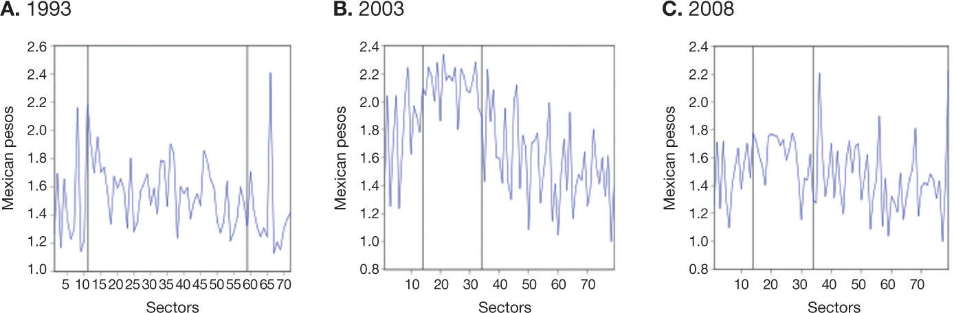
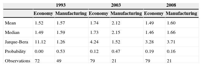
Using all the available information, we measure backward linkages, in first place the direct ones, that is, the so-called matrix A of coefficients, and in second place the direct and indirect ones, or total, the so-called Leontief inverse-matrix. Before showing the total backward linkages results, it is worth noting a caveat. The design of aggregation levels in the matrices is different. Therefore, the temporal comparison related with manufacturing should be taken with caution, to the extent it is well known that the aggregation plays a role in these kind of exercised (Fig. 16; Tables 4 and 5).

Fig. 16.

Direct and indirect linkages in the Mexican economy, internal matrices, 1993, 2003 and 2008.

Source: own calculations using data from the National Accounts System, INEGI.

Table 4.

Direct and indirect linkages in the Mexican economy and Manufacturing sector, internal matrices, Mexican pesos, 1993, 2003 and 2008.

	1993		2003		2008
	Economy	Manufacturing	Economy	Manufacturing	Economy	Manufacturing
Mean	1.52	1.57	1.74	2.12	1.49	1.60
Median	1.49	1.59	1.73	2.15	1.46	1.66
Jarque-Bera	11.12	1.26	4.24	1.52	3.28	3.71
Probability	0.00	0.53	0.12	0.47	0.19	0.16
Observations	72	49	79	21	79	21

Source: own calculations using data from the National Accounts System, INEGI.

Table 5.

Direct and indirect linkages in the Mexican economy and Manufacturing sector, internal matrices, ratios, 1993, 2003 and 2008.

Manufacturing/Economy
	1993	2003	2008
Mean	1.03	1.22	1.07
Median	1.07	1.24	1.14

Source: own calculations using data from the National Accounts System, INEGI.

The economic activities between the lines in the figure (Fig. 17) are the manufacturing ones. Therefore, in terms of its (mean and median) linkages, it is clear the relevant role of the manufacturing as a whole. Both in absolute and relative terms the year 2003 represents a step, that is to say, internal linkages observed their peak in the year 2003. In other words, absolute and relative values for the years 1993 and 2008 are similar. In conclusion, internal linkages won until 2003 were lost at the end of the reporting period (Tables 6 and 7).

Fig. 17.

Direct and indirect linkages in the Mexican Economy, total economy matrices, 1993, 2003 and 2008.

Source: own calculations using data from the National Accounts System, INEGI.

Table 6.

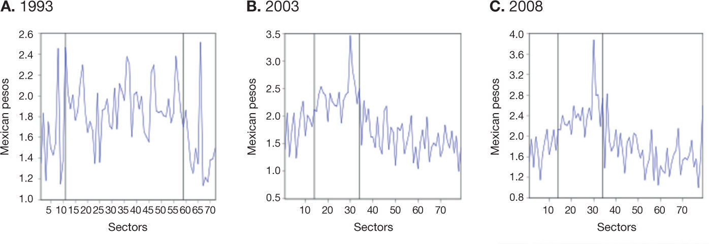
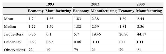
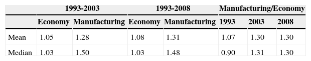
Direct and indirect linkages, Mexican economy and manufacturing sector, total economy matrices, Mexican pesos, 1993 and 2003.

	1993		2003		2008
	Economy	Manufacturing	Economy	Manufacturing	Economy	Manufacturing
Mean	1.74	1.86	1.83	2.38	1.89	2.44
Median	1.77	1.59	1.82	2.39	1.81	2.36
Jarque-Bera	0.76	0.1	5.7	19.46	20.96	44.17
Probability	0.68	0.95	0.06	0.00	0.00	0.00
Observations	72	49	79	21	79	21

Source: own calculations using data from the National Accounts System, INEGI.

Table 7.

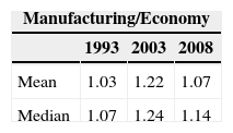
Direct and indirect linkages, Mexican economy and manufacturing sector, total economy matrices, ratios, 1993 and 2003.

	1993-2003		1993-2008		Manufacturing/Economy
	Economy	Manufacturing	Economy	Manufacturing	1993	2003	2008
Mean	1.05	1.28	1.08	1.31	1.07	1.30	1.30
Median	1.03	1.50	1.03	1.48	0.90	1.31	1.30

Between 1993 and 2003 and 2008, total linkages of the Mexican economy were stable, to be precise, based on medians its ratio was, repeatedly, 1.03. In contrast, in the case of the manufacturing the ratio jumped to a figure of 1.50 in 2003 and 1.48 in 2008. As a result, the relative ratios increased between the analyzed period. If we observe the total linkages from medians, the jump is evident, from 0.90 to 1.30. In this sense, the towing capacity of manufacturing sector over the Mexican economy would be a larger one if the manufacturing imports penetration had not been so intense since the trade liberalization. This complex stylized fact is partially explained by the existence of inefficient investment sequences during the analyzed period. Once again, this situation constitutes an opportunity area for the public agents and the private sector.

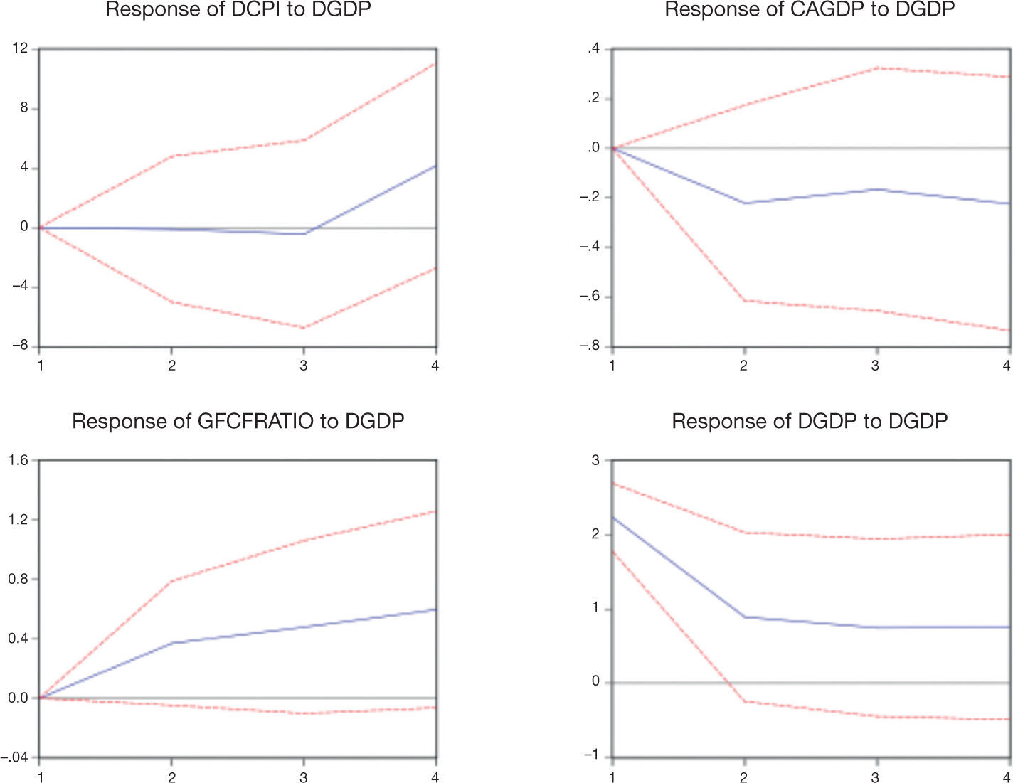
Conclusions

Our complex stylized facts are sets of information given in isolation, that is to say, are not parts of a complete economic model. However, as a cherry on the cake, we estimated a VAR model using the following variables: current account as a percentage of GDP (CAGDP), rate of inflation (DCPI), gross fixed capital formation as a percentage of GDP (GFCFratio), and the economic growth rate (DGDP). By the way, the order of the variables in the VAR was determined by our previous statistical analysis. In the Appendix we show the several tests used in order to verify its statistical adequacy. As in the case of the Granger causality tests that we have already talked about, our VAR conveniently involved stationary variables –which allowed us to avoid the problem of spurious results as a consequence of the presence of trend components. Bearing in mind that “if there is a reaction of one variable to an impulse in another variable we may call the latter casual the former” (Lütkepohl, 1991:43), the next figure (Fig. 18) shows the impulse response analysis relevant to our discussion.

Fig. 18.

Response to Cholesky one S.D. innovations (±2 S.E.), VAR model with four lags, 1960-2012.

Source: own caculations using data from the Balanced of Payments, Mexican Central Bank and the National Accounts System, INEGI.

As expected based on our proposed Hirschmanian facts, the reaction of inflation to the economic growth rate is null, that is to say, there is not a causal link between both variables; the reaction of the current account is negative, so we would better improve our export capabilities and reduce our import necessities; and the reaction of investment is positive –the so-called acceleration effect. The effect of the GDP on itself recalls us that the path of an economy may be in a positive one or a vicious one. I believe that the Mexican economy is trapped in the second case since long ago.

It seems that in Mexico, among other countries, decision makers suffer a sort of “fear of growing”. The complex stylized facts listed constitute a home remedy to attack such an unfounded fear.

From our Hirschmanian perspective, with heterodox touches, the set of economic policies should prioritize jointly, and without exception, the following goals:

• •

  Foster economic growth to bring it closer to its potential (grow, grow and grow is the mantra).

• •

  Increase the efficiency of both, public and private investment, in order to raise internal linkages, improve the current account sustainability, and reduce the external financing as a proportion of the current account.

• •

  Make protagonist to the manufacturing sector.

Without a doubt, the credibility of the Mexican Central Bank finally reached. It constitutes an historical achievement. Definitely, this institution has to maintain the inflation-free environment but also have to rescale some of their actions. According to our complex stylized facts, for example, there is not a contradiction between reduce the reference interest rate and the pursuit of its goal (reduce it, reduce it and reduce it is the mantra). Another issue is the related with the regulation of private banks. For the writer it is unclear its role and responsibilities, facing the Commission Banking and Securities, among other institutional participants. Despite the Mexican macroeconomic stability, with an inflation-free environment, the existence of an adequate number of banking competitors, and a benchmark interest rate of just a few percentage points, the credit to private agents in Mexico is scarce and extremely expensive. Since long ago, the only thing that is clear in consensus is the harmful role of the financial system in the Mexican economy (among others, Hanson, 2010; Kehoe & Ruhl, 2010).^o

To some extent, the role of the exchange rate policy has been misunderstanding. As any key price constitutes a nominal anchor, and the super-peso may give us all a spurious purchasing power, but also influences the Mexican competitiveness. On one hand, one micro-economist would say that competitiveness is a matter of the firm. On the other hand, one way to support the proposed goals is to avoid overvaluation of the peso against the dollar. Indeed, the real effects of the overvalued peso are difficult to notice in the short run but are disastrous in the long run. Needless to say about the required consistency between the set of implemented policies in order to achieve our goals.

Finally, in our country has been implemented, implicitly and explicitly, industrial policy, at any level (National, State and Municipal, see Guerrero, 2012). Our crown jewel, the automobile industry, has developed in part through support programs implemented along the decades. Other success stories are computer and pharmaceutical industries. However, in order to reach the proposed goals, industrial policy must be upgraded. Certainly we need more champions and both, public and private agent, need to choose them without hesitation.

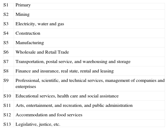
Appendix

Table 1A Sectors of the Mexican Economy.

S1	Primary
S2	Mining
S3	Electricity, water and gas
S4	Construction
S5	Manufacturing
S6	Wholesale and Retail Trade
S7	Transportation, postal service, and warehousing and storage
S8	Finance and insurance, real state, rental and leasing
S9	Professional, scientific, and technical services, management of companies and enterprises
S10	Educational services, health care and social assistance
S11	Arts, entertainment, and recreation, and public administration
S12	Accommodation and food services
S13	Legislative, justice, etc.

Source: National Accounts System, INEGI.

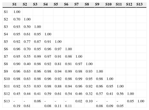
Table 2A Correlation coefficients between sectors, in levels.

	S1	S2	S3	S4	S5	S6	S7	S8	S9	S10	S11	S12	S13
S1	1.00
S2	0.70	1.00
S3	0.93	0.50	1.00
S4	0.95	0.61	0.95	1.00
S5	0.92	0.77	0.87	0.91	1.00
S6	0.96	0.70	0.95	0.96	0.97	1.00
S7	0.95	0.55	0.99	0.97	0.91	0.98	1.00
S8	0.90	0.40	0.98	0.92	0.81	0.91	0.97	1.00
S9	0.96	0.63	0.96	0.98	0.94	0.99	0.98	0.93	1.00
S10	0.98	0.63	0.98	0.96	0.92	0.98	0.99	0.95	0.98	1.00
S11	0.92	0.53	0.93	0.98	0.88	0.94	0.96	0.92	0.96	0.95	1.00
S12	0.45	0.44	0.41	0.59	0.61	0.54	0.46	0.32	0.57	0.41	0.56	1.00
S13	-0.19	-0.61	0.06	-0.08	-0.11	-0.11	0.02	0.10	-0.08	-0.09	-0.05	0.05	1.00

Source: own calculations using data from the National Accounts System, INEGI.

Table 3A Correlation coefficients between sectors, in growth rates.

	DS1	DS2	DS3	DS4	DS5	DS6	DS7	DS8	DS9	DS10	DS11	DS12	DS13
DS1	1.00
DS2	0.27	1.00
DS3	0.23	–0.05	1.00
DS4	0.26	0.37	0.42	1.00
DS5	0.22	0.56	0.42	0.70	1.00
DS6	0.21	0.55	0.40	0.79	0.95	1.00
DS7	0.28	0.30	0.55	0.80	0.83	0.83	1.00
DS8	0.19	–0.33	0.35	0.25	0.13	0.23	0.29	1.00
DS9	0.27	0.29	0.45	0.75	0.74	0.81	0.82	0.32	1.00
DS10	0.27	–0.12	0.39	0.31	0.20	0.23	0.38	–0.06	0.47	1.00
DS11	0.12	0.13	0.28	0.83	0.58	0.64	0.84	0.23	0.64	0.33	1.00
DS12	0.29	0.35	0.46	0.86	0.80	0.87	0.92	0.41	0.83	0.33	0.79	1.00
DS13	–0.06	–0.27	0.38	0.24	0.27	0.26	0.40	0.34	0.15	0.06	0.29	0.38	1.00

Source: own calculations using data from the National Accounts System, INEGI.

Table 4A Granger causality test, inflation and economic growth.

Sample: 2007M01 2013M12
Null Hypothesis	F-Statistic	Prob.
Lags: 1
DCPI does not Granger Cause DGEAI	7.01591	0.0100
DGEAI does not Granger Cause DCPI	0.01547	0.9014
Lags: 2
DCPI does not Granger Cause DGEAI	3.31914	0.0424
DGEAI does not Granger Cause DCPI	0.81261	0.4482
Lags: 3
DCPI does not Granger Cause DGEAI	2.93334	0.0403
DGEAI does not Granger Cause DCPI	0.63025	0.5982
Lags: 4
DCPI does not Granger Cause DGEAI	2.46124	0.0550
DGEAI does not Granger Cause DCPI	1.04960	0.3895
Lags: 5
DCPI does not Granger Cause DGEAI	2.20252	0.0668
DGEAI does not Granger Cause DCPI	1.04187	0.4023
Lags: 6
DCPI does not Granger Cause DGEAI	2.22587	0.0547
DGEAI does not Granger Cause DCPI	1.11564	0.3659
Lags: 7
DCPI does not Granger Cause DGEAI	3.28525	0.0060
DGEAI does not Granger Cause DCPI	1.15912	0.3429
Lags: 8
DCPI does not Granger Cause DGEAI	2.61471	0.0187
DGEAI does not Granger Cause DCPI	1.03301	0.4253
Lags: 9
DCPI does not Granger Cause DGEAI	2.88389	0.0091
DGEAI does not Granger Cause DCPI	1.24145	0.2955
Lags: 10
DCPI does not Granger Cause DGEAI	3.13974	0.0046
DGEAI does not Granger Cause DCPI	1.30595	0.2596
Lags: 11
DCPI does not Granger Cause DGEAI	2.99202	0.0059
DGEAI does not Granger Cause DCPI	1.10055	0.3871
Lags: 12
DCPI does not Granger Cause DGEAI	2.12544	0.0411
DGEAI does not Granger Cause DCPI	1.18837	0.3288

Source: own calculations using data from the National Accounts System, INEGI.

Table 5A Granger causality test, current account as % of GDP and economic growth.

Sample: 1960 2012
Null Hypothesis	F-Statistic	Prob.
Lags: 1
CAGDP does not Granger Cause DGDP	2.18770	0.1457
DGDP does not Granger Cause CAGDP	10.1214	0.0026
Lags: 2
CAGDP does not Granger Cause DGDP	3.02537	0.0585
DGDP does not Granger Cause CAGDP	3.98872	0.0254
Lags: 3
CAGDP does not Granger Cause DGDP	2.19315	0.1030
DGDP does not Granger Cause CAGDP	3.62781	0.0204

Source: own calculations using data from the Balanced of Payments, Mexican Central Bank and the National Accounts System, INEGI.

Table 6A Granger causality test, investment ratio and economic growth.

Sample: 1960 2012
Null Hypothesis	F-Statistic	Prob.
Lags: 2
GFCFRATIO does not Granger Cause DGDP	3.49056	0.0390
DGDP does not Granger Cause GFCFRATIO	0.87252	0.4248
Lags: 4
GFCFRATIO does not Granger Cause DGDP	1.10754	0.3668
DGDP does not Granger Cause GFCFRATIO	0.83180	0.5132
Lags: 6
GFCFRATIO does not Granger Cause DGDP	0.74157	0.6201
DGDP does not Granger Cause GFCFRATIO	1.04264	0.4160
Lags:2
DGDP does not Granger Cause BUILDINGSRATIO	0.36391	0.6970
BUILDINGSRATIO does not Granger Cause DGDP	0.08747	0.9164
Lags:4
DGDP does not Granger Cause BUILDINGSRATIO	0.30185	0.8749
BUILDINGSRATIO does not Granger Cause DGDP	0.15984	0.9573
Lags:6	0.91119	0.4991
DGDP does not Granger Cause BUILDINGSRATIO	0.14865	0.9880
BUILDINGSRATIO does not Granger Cause DGDP
Lags:2
MACHINERYRATIO does not Granger Cause DGDP	4.99559	0.0110
DGDP does not Granger Cause MACHINERYRATIO	0.17030	0.8440
Lags:4
MACHINERYRATIO does not Granger Cause DGDP	1.61921	0.1888
DGDP does not Granger Cause MACHINERYRATIO	0.70452	0.5937
Lags:6
MACHINERYRATIO does not Granger Cause DGDP	1.05391	0.4094
DGDP does not Granger Cause MACHINERYRATIO	1.33794	0.2685

Source: own calculations using data from the National Accounts System, INEGI. In order to determine the VARs lags the following test were applied: LR: sequential modified LR test statistic, FPE: Final prediction error, AIC: Akaike information criterion, SC: Schwarz information criterion, and HQ: Hannan-Quinn information criterion. We also applied a set of tests to verify the no-autocorrelation, the normality, the no-heteroskedasticity, weak exogeneity, and the stability condition of the VARs.

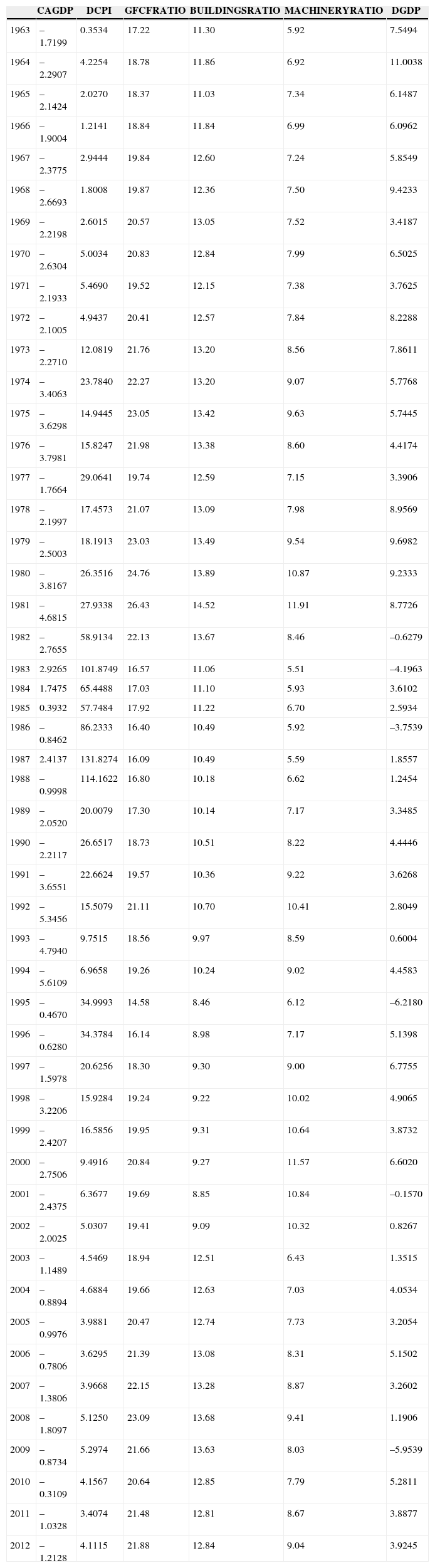
Table 7A Database.

	CAGDP	DCPI	GFCFRATIO	BUILDINGSRATIO	MACHINERYRATIO	DGDP
1963	–1.7199	0.3534	17.22	11.30	5.92	7.5494
1964	–2.2907	4.2254	18.78	11.86	6.92	11.0038
1965	–2.1424	2.0270	18.37	11.03	7.34	6.1487
1966	–1.9004	1.2141	18.84	11.84	6.99	6.0962
1967	–2.3775	2.9444	19.84	12.60	7.24	5.8549
1968	–2.6693	1.8008	19.87	12.36	7.50	9.4233
1969	–2.2198	2.6015	20.57	13.05	7.52	3.4187
1970	–2.6304	5.0034	20.83	12.84	7.99	6.5025
1971	–2.1933	5.4690	19.52	12.15	7.38	3.7625
1972	–2.1005	4.9437	20.41	12.57	7.84	8.2288
1973	–2.2710	12.0819	21.76	13.20	8.56	7.8611
1974	–3.4063	23.7840	22.27	13.20	9.07	5.7768
1975	–3.6298	14.9445	23.05	13.42	9.63	5.7445
1976	–3.7981	15.8247	21.98	13.38	8.60	4.4174
1977	–1.7664	29.0641	19.74	12.59	7.15	3.3906
1978	–2.1997	17.4573	21.07	13.09	7.98	8.9569
1979	–2.5003	18.1913	23.03	13.49	9.54	9.6982
1980	–3.8167	26.3516	24.76	13.89	10.87	9.2333
1981	–4.6815	27.9338	26.43	14.52	11.91	8.7726
1982	–2.7655	58.9134	22.13	13.67	8.46	–0.6279
1983	2.9265	101.8749	16.57	11.06	5.51	–4.1963
1984	1.7475	65.4488	17.03	11.10	5.93	3.6102
1985	0.3932	57.7484	17.92	11.22	6.70	2.5934
1986	–0.8462	86.2333	16.40	10.49	5.92	–3.7539
1987	2.4137	131.8274	16.09	10.49	5.59	1.8557
1988	–0.9998	114.1622	16.80	10.18	6.62	1.2454
1989	–2.0520	20.0079	17.30	10.14	7.17	3.3485
1990	–2.2117	26.6517	18.73	10.51	8.22	4.4446
1991	–3.6551	22.6624	19.57	10.36	9.22	3.6268
1992	–5.3456	15.5079	21.11	10.70	10.41	2.8049
1993	–4.7940	9.7515	18.56	9.97	8.59	0.6004
1994	–5.6109	6.9658	19.26	10.24	9.02	4.4583
1995	–0.4670	34.9993	14.58	8.46	6.12	–6.2180
1996	–0.6280	34.3784	16.14	8.98	7.17	5.1398
1997	–1.5978	20.6256	18.30	9.30	9.00	6.7755
1998	–3.2206	15.9284	19.24	9.22	10.02	4.9065
1999	–2.4207	16.5856	19.95	9.31	10.64	3.8732
2000	–2.7506	9.4916	20.84	9.27	11.57	6.6020
2001	–2.4375	6.3677	19.69	8.85	10.84	–0.1570
2002	–2.0025	5.0307	19.41	9.09	10.32	0.8267
2003	–1.1489	4.5469	18.94	12.51	6.43	1.3515
2004	–0.8894	4.6884	19.66	12.63	7.03	4.0534
2005	–0.9976	3.9881	20.47	12.74	7.73	3.2054
2006	–0.7806	3.6295	21.39	13.08	8.31	5.1502
2007	–1.3806	3.9668	22.15	13.28	8.87	3.2602
2008	–1.8097	5.1250	23.09	13.68	9.41	1.1906
2009	–0.8734	5.2974	21.66	13.63	8.03	–5.9539
2010	–0.3109	4.1567	20.64	12.85	7.79	5.2811
2011	–1.0328	3.4074	21.48	12.81	8.67	3.8877
2012	–1.2128	4.1115	21.88	12.84	9.04	3.9245

Source: own calculations using data from the National Accounts System, INEGI.