Analizamos las preferencias de un subastador con aversión al riesgo en diferentes modelos de subasta con participantes neutrales al riesgo y simétricos. Obtenemos el valor en riesgo (VaR) de los ingresos del subastador en los mecanismos de subasta que pertenecen a una familia paramétrica que incluye dos mecanismos clásicos: la subasta de primer precio y la subasta de segundo precio. Mediante el cálculo del VaR de los ingresos, un subastador puede estimar la cantidad que se perderá dentro de un nivel de confianza dado, dependiendo del número de participantes y del mecanismo de subasta elegido. La novedad de este artículo es el cálculo del VaR de los ingresos del subastador en algunos mecanismos de subasta comunes, que producen los mismos ingresos esperados y que incluyen la subasta de primer precio y la subasta de segundo precio, así como los siguientes mecanismos: subasta «Santa Claus», subasta «Perdedores Tristes» y subasta «Todos pagan». Describimos cómo cuantificar la pérdida máxima de un subastador con una probabilidad dada. Estudiamos el valor en riesgo del subastador como un criterio para determinar qué subastas se adaptarían mejor a los intereses del subastador.
We analyze the preferences of a risk-averse auctioneer over several auction mechanisms with risk-neutral and symmetric bidders. We obtain the value at risk (VaR) for auctioneer revenue in auction mechanisms belonging to a parametric family which includes two classic mechanisms, the first¿price auction and second¿price auction. By calculating the VaR for revenue an auctioneer can estimate the amount that will be lost within a given confidence level, depending on the number of bidders and the auction mechanism chosen. The contribution of this paper is the calculation of the VaR for auctioneer revenue in some common auction mechanisms that yield the same expected revenue, including first¿price auction and second-price auction and the following mechanisms: Santa Claus auction, sad-loser auction and all-pay auction. We describe how to quantify the maximum loss for an auctioneer at a given probability. We study the value at risk of the auctioneer as a criterion to determine which auctions would best suit the auctioneer's interests.
1. Introduction
Under some conditions, when a single object is auctioned, two classical auction mechanisms, the first¿price auction (FPA) and second-price auction (SPA), generate the same expected payment by bidders and therefore the same expected revenue for the auctioneer (Vickrey, 1961). In fact, the Revenue Equivalence Theorem (Myerson, 1981) is verified if two auction mechanisms have the same allocation rule and produce the same bidder payment with valuation 0. If the auctioneer takes only the expected revenue into account (risk-neutral auctioneer) then every auction mechanism that satisfies the Revenue Equivalence Theorem is equally attractive to the auctioneer. However, every risk-averse auctioneer would prefer the auction mechanism with the lowest variance (assuming, of course, that the bidders are risk-neutral).
To establish a preference between the classical auction mechanisms, their variability (usually their variance) is often compared. Vickrey (1961) calculated the variance for FPA and English auctions. Waehrer et al. (1998) proved that a risk-averse auctioneer prefers FPA to SPA and SPA to an English auction. Beltrán and Santamaría (2006) used simulation to analyze the variation for several auction mechanisms with the same expected revenue. Krishna (2002) proved that the price distribution in SPA is a mean-preserving spread of the price distribution in FPA.
The main problem with variance is that it does not indicate the direction of revenue deviations: revenue can be volatile and can suddenly take high values. An auctioneer is not affected if revenue is higher than expected; however, much lower than expected revenues could lead to bankruptcy. Hence, we are interested in obtaining a measure of the risk of losses for each auction mechanism.
In the literature we can find a number of papers on the optimal choice or design of auctions, usually from the point of view of the expected revenue (see, for example, Myerson, 1981; Riley and Samuelson, 1981). For this reason, if the auctioneer only takes into account the expected revenue, then every auction mechanism satisfying the Revenue Equivalence Theorem is identical for her. Consequently, the auctioneer should take into account other criteria when making her decision. A possible criterion is collusion (Robinson, 1985), another is variability (Vickrey, 1961), and other criteria could also be used. We aim at giving the auctioneer a second criterion for choosing an appropriate auction mode. Therefore, the original contribution of this paper is the analysis of risk measures applied to auctions.
Value at risk (VaR) is a measure of the worst loss at a given confidence level and reflects how much can be lost with respect to expected revenue at a certain probability (Holton, 2004). We must bear in mind that although expected auctioneer revenue is a good long-term indicator, a sudden and unexpected decrease in actual revenue could lead to bankruptcy. The VaR for auctioneer revenue at a given confidence level quantifies the maximum loss compared to expected revenue. Thus, if an auctioneer knows in advance that the possible maximum loss is greater than what can be absorbed economically, the auction mechanism can be changed or the number of bidders can be increased to reduce this risk. We therefore believe that VaR can be very useful for auctions that, despite being equally attractive in terms of expected revenue, are different in terms of loss risk.
The contribution of this paper is the calculation of the VaR for auctioneer revenue in some common auction mechanisms that yield the same expected revenue, including FPA and SPA and the following mechanisms: Santa Claus auction (SCA), sad-loser auction (SLA) and all-pay auction (APA). Thus, we quantify the maximum loss for an auctioneer at a given probability.
We assume the following hypotheses:
There are n ≥ 2 risk-neutral bidders competing to buy a single object. The valuation of bidder iÎ {1, ..., n} is qi. Each type qi, which is information known only to bidder i, is an independent realization of a uniformly distributed continuous random variable Qi in [0,1]. Only bidder i observes the realization of qi, which reflects the uncertainty that bidder j has about the valuation of bidder i.
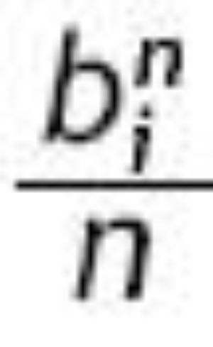
Each bidder i Î {1, ..., n} simultaneously and independently submits a bid bi Î [0,1] specifying the maximum unit-price offer at which he is willing to buy the object.
A strategy for bidder i Î {1, ..., n} is a function bi(qi): [0,1]→ [0,1].
We refer to this model as the symmetric model.
Once the auctioneer has received all the bids, the highest bidder wins the object. The price paid by each bidder depends on the auction mechanism adopted for the transaction. Each aspect of this model and the auction mechanism chosen is assumed to be common knowledge. This situation is modeled as a single-object auction as an n¿person game with incomplete information (Harsanyi, 1967-1968) under the assumption of symmetric and risk-neutral bidders with independent and uniformly distributed [0,1] values.
The rest of the paper is organized as follows. In Section 2 we define the parametric family of auction mechanisms for selling one object, and obtain the Bayesian Nash equilibrium for each auction mechanism in the parametric family. In Section 2.1. we obtain the distribution function of the random variable that gives the auctioneer revenue at the equilibrium in each auction mechanism in the parametric family, we prove that each auction mechanism in the parametric family verifies a revenue equivalence theorem and we calculate the variance and the VaR of the auctioneer revenue. In Section 2.2. we give the VaR for auctioneer revenue for different numbers of bidders and different auction mechanisms. In Section 3 we analyze other auction mechanisms by comparing them with regard to their VaR for auctioneer revenue. Finally, Section 4 gives the conclusions.
2. First¿second¿price auction family
The two classic auction mechanisms are FPA and SPA. In FPA the winner pays the winning bid bi. In SPA the winner pays the second highest bid. Here we consider a parametric family of auction mechanisms that contains FPA and SPA as particular cases. This family, called the first¿second¿price parametric family (FSP), is a set of auction mechanisms Ag whose profit function for bidder i is:
That is, if i bids the highest amount, then i buys the object and possibly pays different prices: an amount y at price bi and the remaining amount (1 - g) at the second highest bid, maxj≠i bj. In particular, if g = 1 we have the FPA and if g = 0, we have the SPA.
We can assume, given the symmetry of the model, that bi(qi) = b(qi) is the bid function used in the equilibrium by all bidders where b(qi) is a strictly monotone and differentiable function. The following proposition gives the Bayesian Nash equilibrium for any auction mechanism belonging to FSP.
Proposition 1. If the hypotheses for the symmetric model are verified and an auction mechanism AgÎ FSP is used, then the unique symmetric Bayesian Nash equilibrium _bg(q1),...,bg(qn)+ with the condition limqi→0+bg(qi) = 0, is:
Proof. Let g = Max{Q1, ... , Qi-1, Qi+1, ... ,Qn} be the highest-order statistic for the other n - 1 bidder types. Then the profit for bidder i is:
Bidder i knows his own type qi, but g is a random variable, so the expected profit for bidder i is given by:
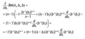
Thus, bi is the best bid for bidder i if it maximizes the expected profit, given type qi. The derivative with respect to bi is:
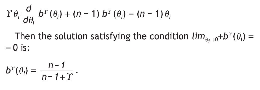
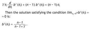
As b-1(bi) = qi Û bi = b(qi), replacing and setting the above equation equal to zero, we obtain the following differential equation:
2.1. Statistical properties of the revenue
Once the Bayesian Nash equilibrium has been determined, we can calculate the distribution, expectation, variance and VaR of the auctioneer revenue. It is easy to find that the expected revenue is independent of g , which means that there is a revenue equivalence result for every auction mechanism belonging to FSP.
Let Xg be the random variable that gives the auctioneer revenue at equilibrium in an auction mechanism AgÎ FSP:
where g is the highest-order and Z is the second-highest-order statistic of {Q1, ... ,Qn}. The variable Xg is distributed in
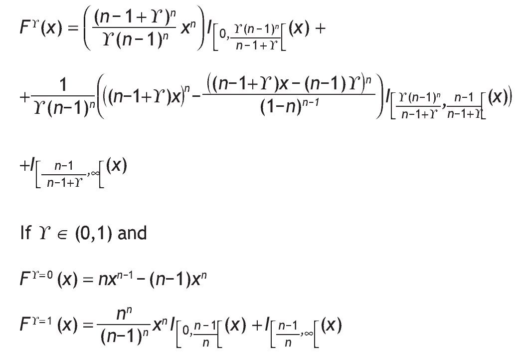
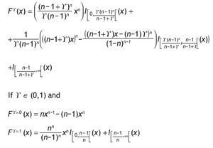
and its probability distribution function is given by:
Then the expected auctioneer revenue is:
If the auctioneer takes into account only expected revenue (risk-neutral auctioneer), then every auction mechanism belonging to FSP is equally attractive. However, every risk-averse auctioneer could prefer the auction mechanism with lowest variance (assuming, of course, that the bidders are risk-neutral).
The variance of the auctioneer revenue is:
This decreases in g and therefore the auction mechanism belonging to FSP with minimum revenue variance is the FPA.
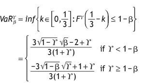
The main problem with variance is that it does not indicate the sign of revenue deviations: revenue can be volatile and suddenly take high values. Given a confidence level β, the VaR for auctioneer revenue is the smallest number k such that the probability that the difference between expected and actual revenue (the loss) is less than k and greater than β in auction mechanism Ag :
Example
If there are two bidders (n = 2).
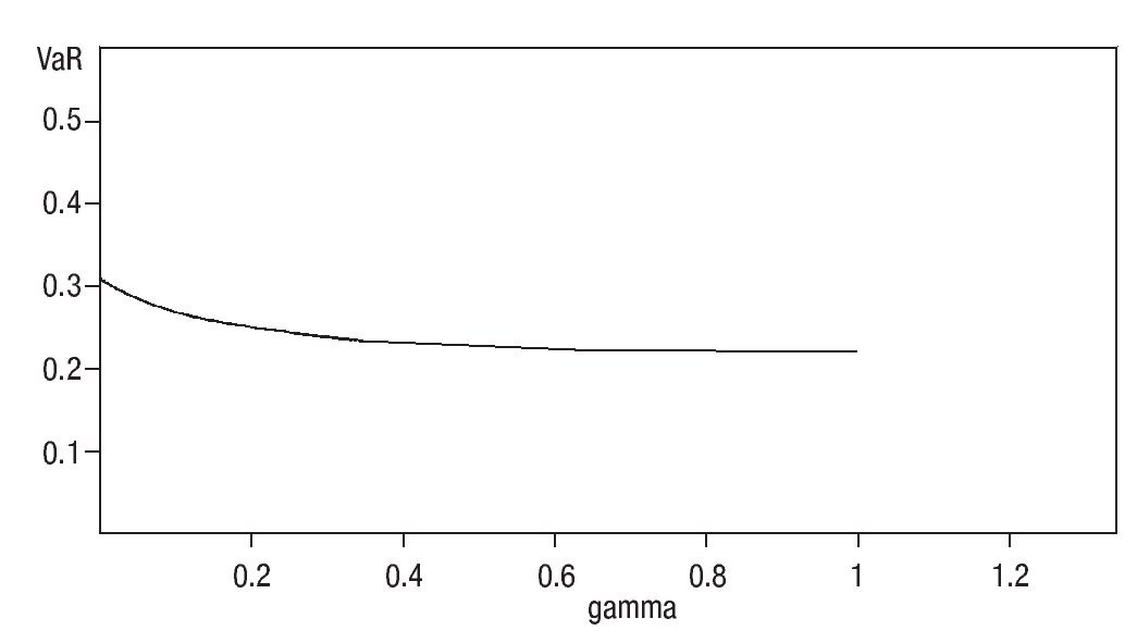
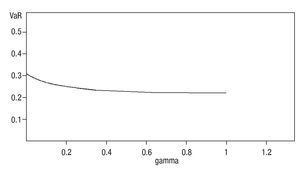
Figure 1 shows VaR for two bidders at a confidence level of 0.95 and gÎ [0,1].
Figure 1VaRgβ for n = 2.
2.2. Numerical results
In this section we give the VaR for auctioneer revenue for different numbers of bidders and different auction mechanisms of parameter g . We take two typical confidence levels, 0.95 and 0.99. We also compute the relative VaR (RVaR) given by:
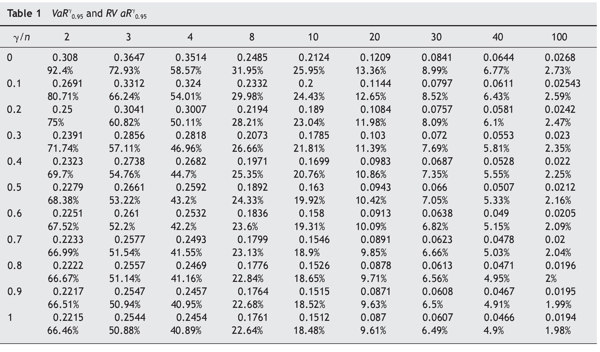
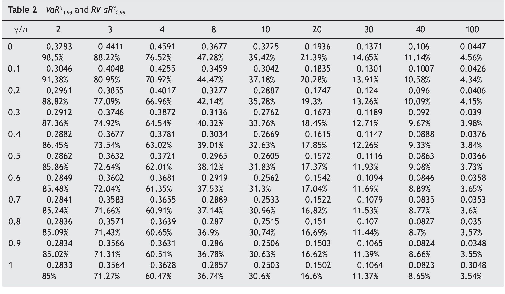
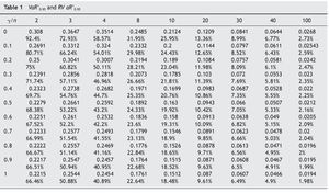
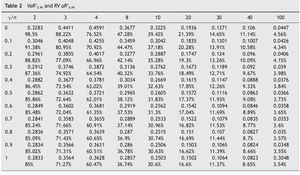
Tables 1 and 2 list values of VaR and RVaR for different auction mechanisms and numbers of bidders for confidence levels of 0.95 and 0.99 respectively.
The auction mechanisms belonging to FSP with the lowest and highest VaR for revenue are FPA (g = 1) and SPA (g = 0) respectively. For example, if the number of bidders is n = 4, with probability ≥ 0.95, the difference between expected and actual revenue is ≤ 0.3514 in SPA and ≤ 0.2454 in FPA. For the same probability level, FPA yields smaller losses for the auctioneer. The expected revenue in this case is 3/5, so at the 95% confidence level the loss will not exceed 58.57% in SPA nor exceed 40.89% in FPA.
The VaR for auctioneer revenue tends to 0 when the number of bidders increases in all auction mechanisms belonging to FSP, while revenue tends to 1.
By calculating VaR, an auctioneer can estimate at a given confidence level the maximum amount that can be lost, depending on the number of bidders and the auction mechanism chosen.
3. Other auction mechanisms
There are of course endless auction mechanisms. We analyzed a parametric family containing the two most common, but there are other auction mechanisms that while giving the same expected auctioneer revenue, can yield VaR that is less than that for FPA. This paper shows a method for measuring the risk and thus provides the auctioneer with a second criterion for choosing the most suitable auction mechanism.
Below we consider other auction mechanisms that can be found in different contexts: APA, SLA and SCA. The expected auctioneer revenue is the same as in any auction mechanism belonging to FSP. The VaR for auctioneer revenue for these other mechanisms was obtained by simulation.
3.1. All¿pay auction
In this auction mechanism the highest bidder wins the object but all bidders pay their bid. The profit function for bidder i Î {1, ..., n} is:
It is well known that the symmetric Bayesian Nash equilibrium (bAP(q1), ... , bAP(qn)) is
Let XAP be the random variable that gives the auctioneer revenue in APA:
3.2. Sad¿loser auction
In this auction mechanism, the highest bidder wins the object but pays nothing. All other bidders pay their bids. Then the profit function for bidder i Î {1, ... , n} is:
It is well known that the symmetric Bayesian Nash equilibrium _ bSL(q1), ... , bSL(qn)+ is
Hence let XSL be the random variable that gives the auctioneer revenue in SLA:
where Y(i) is the ith-order statistic for {Q1, ... ,Qn}.
3.3. Santa Claus auction
Finally, in the SCA mechanism the highest bidder wins the object and pays his own bid bi, Î {1, ... , n}, but all bidders receive the amount
. Then the profit function for bidder i is:The symmetric Bayesian Nash equilibrium (bSC(q1),..., bSC(qn)) is given by
Let XSC be the random variable that gives the auctioneer revenue in SCA:
where g is the highest-order statistic for {Q1, ... , Qn}.
3.4. Numerical results
We calculated the sample VaR for the auctioneer revenue in the above three auction mechanisms. For this, each auction mechanism was repeated 100 000 times. Tables 3 and 4 show VaR and RVaR values for the auctioneer revenue for different numbers of bidders in SCA, APA and SLA mechanism at confidence levels of 0.95 and 0.99 respectively.
We can observe that the VaR for auctioneer revenue in SCA tends to 0. In SLA, the VaR for auctioneer revenue is very high and decreases only slightly with increasing competition (for n = 1000, β = 0.95 the RVaR is 98.4%). In APA the VaR for auctioneer revenue is also very high, but seems to increase with competition (for n = 1000, β = 0.95 the RVaR is 91.25%), meaning the auctioneer can have lower VaR with two bidders than with another number of bidders. Menicucci (2009) proved that in APA, if t he type distribution satisfies some specific assumptions, the volatility of auctioneer revenue increases with competition.
4. Conclusions
We analyzed a parametric family of auction mechanisms FSP containing FPA and SPA as particular cases. We assumed hypotheses that included independent and uniformly distributed [0,1] types. We obtained a unique Bayesian Nash equilibrium for each auction mechanism belonging to FSP.
For a risk-neutral auctioneer, every auction mechanism belonging to FSP is equally attractive, but a risk-averse auctioneer would prefer the mechanism with the lowest VaR. We calculated the VaR for auctioneer revenue for the auction mechanisms belonging to FSP.
Calculation of VaR enables the auctioneer to estimate the maximum amount that can be lost at a given confidence level, depending on the number of bidders and the auction mechanism used.
The results could also be useful from another point of view: if an auctioneer knows in advance that the possible maximum loss is greater than what can be absorbed economically, a different auction mechanism can be chosen or the number of bidders can be increased to reduce this risk.
We must bear in mind that although the expected auctioneer revenue is a good long-term indicator, a sudden and unexpected decrease in actual revenue could still lead to bankruptcy. In addition, we considered other auction mechanisms (SLA, APA and SCA).
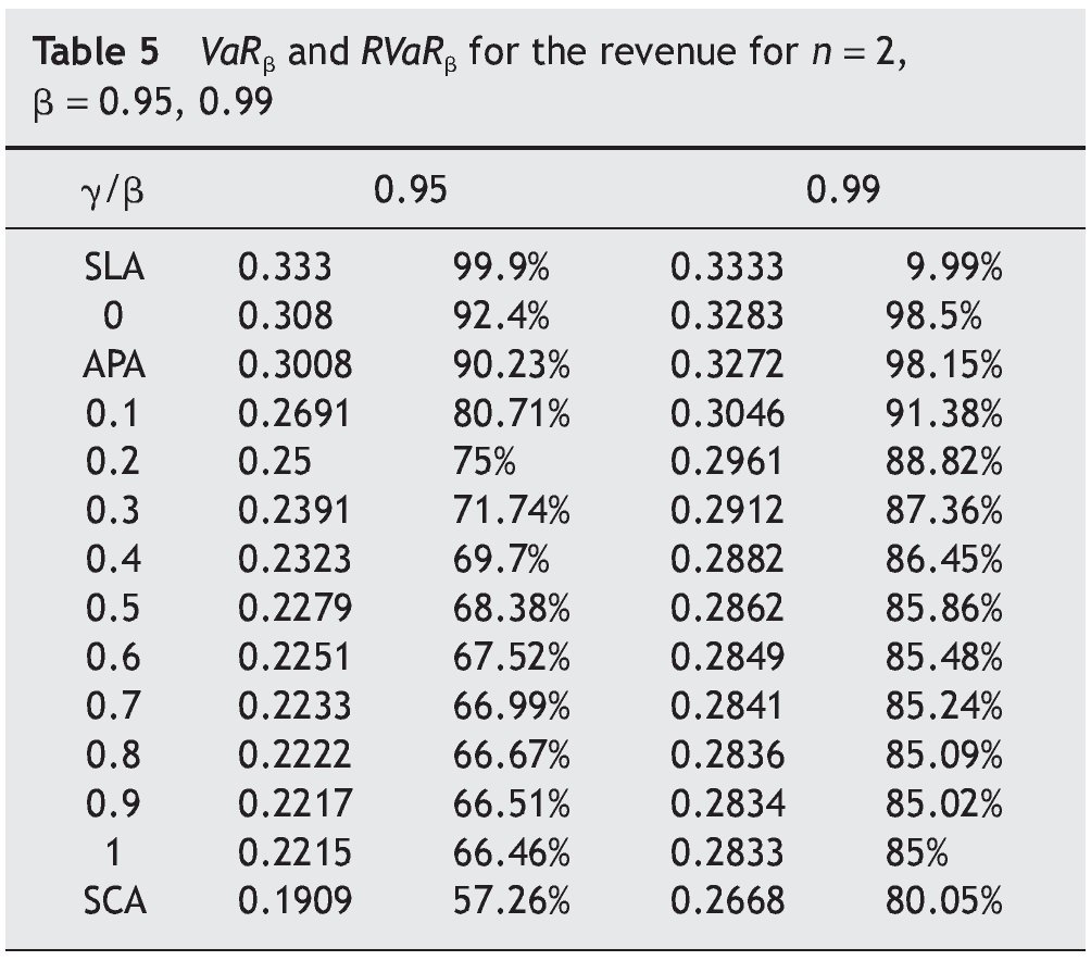
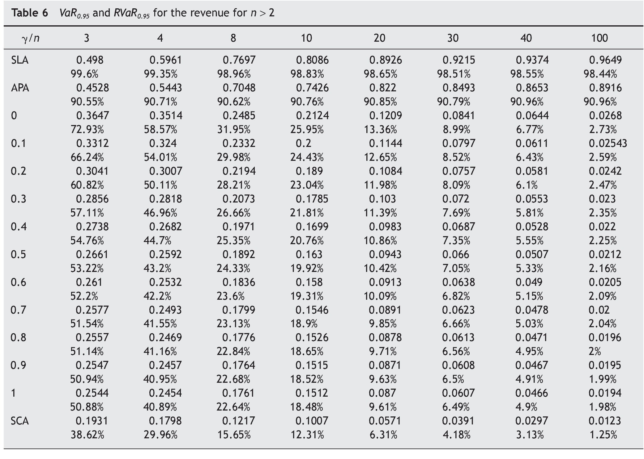
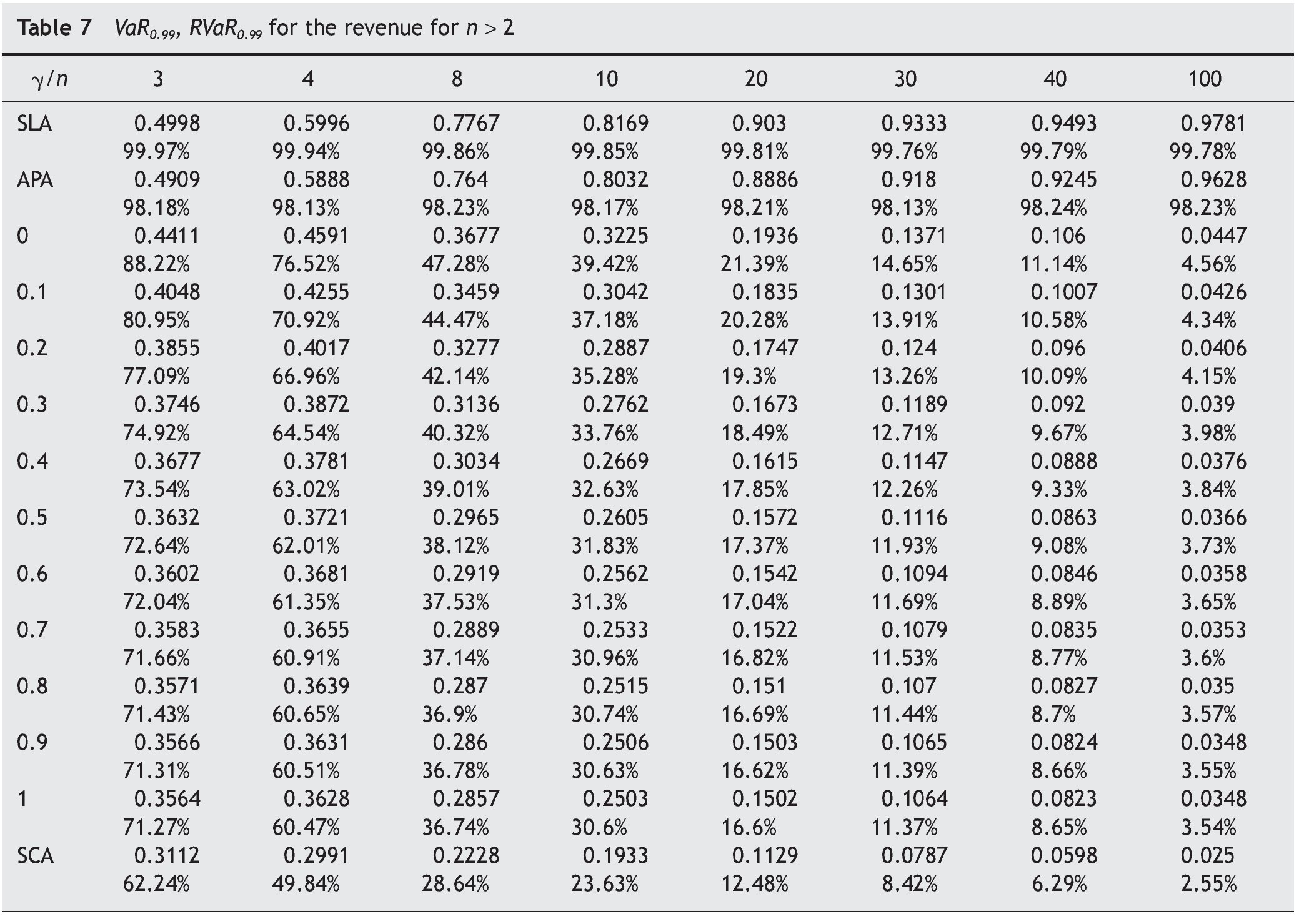
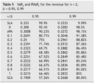
The variance and VaR followed the same order for the auctioneer revenue obtained in the different auction mechanisms considered. If n = 2, the order is SCA < FPA < APA<< SPA < SLA. Table 5 summarizes the VaR and the RVaR values for all auction mechanisms for two bidders and confidence levels β = 0.95 and 0.99. If n > 2, the order is SCA < FPA< < SPA < APA < SLA. Tables 6 and 7 summarize the VaR and RVaR values for all auction mechanisms for different numbers of bidders and confidence levels β = 0.95 and 0.99 respectively.
We can observe that the VaR for auctioneer revenue in SCA tends to 0 when the competition increases, just like the auction mechanisms belonging to the family FSP. In addition, the VaR in SCA is lower than in any auction mechanism belonging to FSP.
SCA has the lowest VaR for auctioneer revenue among all the auction mechanisms analyzed and a VaR for bidder profit equal to 0. In SLA the VaR for auctioneer revenue is very high and only decreases slightly with increasing competition. In APA the VaR for auctioneer revenue is also very high, but seems to increase with competition. This means that the auctioneer can expect a lower VaR with two bidders than with any other number of bidders. Menicucci (2009) proved that if the type distribution satisfies some specific assump¿ tions in APA, the volatility of auctioneer revenue increases with competition.
Acknowledgment
The authors gratefully acknowledge support under Project MTM 2011-27892.
Recibido el 4 de junio de 2012; aceptado el 20 de noviembre de 2012
* Correspondingauthor.
E-mail address:ealonso@upcomillas.es (E. Alonso).
References
Beltrán, F., Santamaría, N., 2006. A measure of the variability of revenue in auctions: a look at the Revenue Equivalence Theorem. Journal of Applied Mathematics and Decision Sciences. Article ID 27417, 1-14.
Harsanyi, J., 1967-1968. Games with Incomplete Information played by Bayesian Players (Parts I-III). Management Science 14, 159-182; 320-334; 486-502.
Holton, G., 2004. Value at risk: Theory and practice. Elsevier Academic Press.
Krishna, V., 2002. Auction theory. Elsevier Academic Press (Chapter 2). Menicucci, D., 2009. Harmful competition in all-pay auctions. Mathematical Social Sciences 58, 110-120.
Myerson, R., 1981. Optimal auction design. Mathematics of Operations Research 6, 58-73.
Riley, J.G., Samuelson, W.F., 1981. Optimal auctions. American Economic Review 71, 381-392.
Robinson, M.S., 1985. Collusion and the choice of auction. Rand Journal of Economics 16, 141-145.
Vickrey, W., 1961. Counterspeculation, auctions and competitive sealed tenders. Journal of Finance 16, 8-37.
Waehrer, K., Harstad, R.M., Rothkopf, M.H., 1998. Auction form preferences of risk-averse bid takers. RAND Journal of Economics 29, 179-192.


