Model for the compressive stress–strain relationship of steel fiber-reinforced concrete for non-linear structural analysis

Abstract

A model for non-linear calculations of steel fiber-reinforced concrete (SFRC) elements in compression is proposed and described technologically. The same curve produced by Eurocode 2 (EC2) is used until compressive strength, although non-dimensional variables refer to fiber concrete parameters. Beyond the peak, we use a parabola that is derived so that the average energy consumption of the material equals this same mean energy obtained from a database comprised of 197 tests. Estimates for the compressive strength of SFRC and the corresponding critical strain are also provided by correlation with the database using the surface response methodology. The total energy consumption of SFRC in compression is approximately four times higher on average than the corresponding energy of the base plain concrete, which is included in the model. Therefore, it can considerably improve the modeling of ductility in SFRC structures.

Resumen

Se propone y se describe, en formato tecnológico, un modelo para el cálculo no-lineal de elementos de hormigón reforzado con fibras de acero (HRFA) en compresión. Hasta el pico de carga, se usa la curva dada por el Eurocódigo 2 (EC2), aunque las variables adimensionales se refieren a los parámetros del hormigón reforzado con fibras. Después del pico, usamos una parábola que se calcula de modo que la energía consumida por el material sea igual al valor de esa misma energía dada por una base de datos compuesta por 197 ensayos. También se proporcionan estimaciones de la resistencia a compresión del HRFA y de la deformación crítica correspondiente, las cuales se obtienen por correlaciones con la base de datos usando la metodología de las superficies de respuesta. La energía consumida por el HRFA en compresión es, como media, unas cuatro veces mayor que la que tendría su matriz sin reforzar, lo cual es reproducido por el modelo. Así, éste puede mejorar considerablemente el modelado de la ductilidad en estructuras de HRFA.

1

Introduction

This technical note describes a model for the compressive stress–strain (σ–ɛ) behavior of steel fiber-reinforced concrete. The model is based on functions obtained from correlations with an extensive database comprised of 197 well-documented SFRC compressive tests [1–20].

The following section describes the σ–ɛ model. Subsequently, we justify the assumptions made to formulate the model and provide a brief description of the database that supports a few of the expressions of the model, together with a short explanation of the response-surface methodology and the process followed in order to obtain the responses.

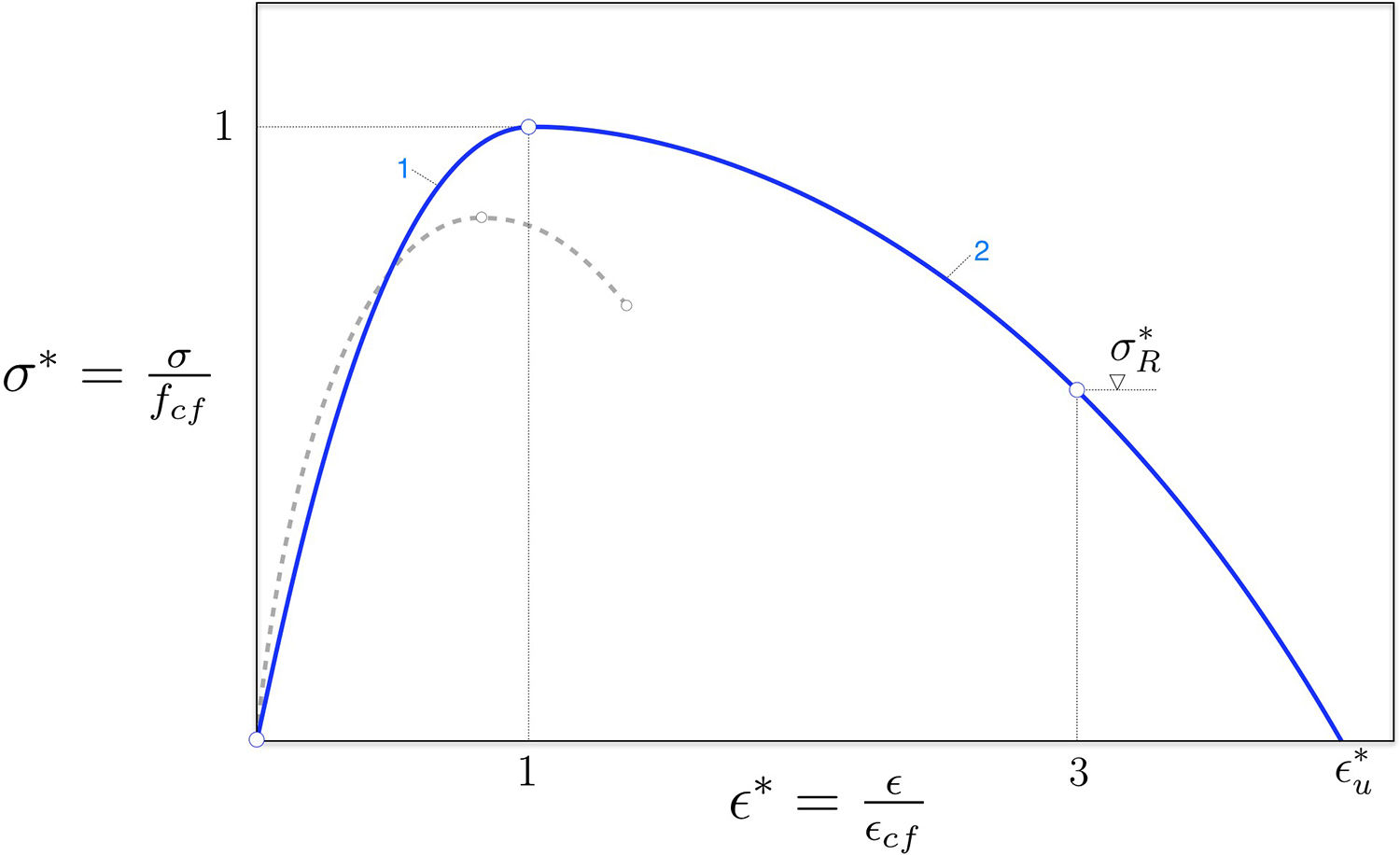
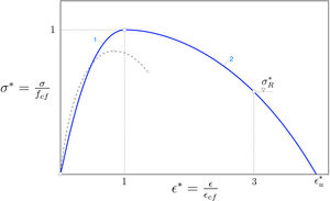
2

σ–ɛ relationship for non-linear structural analysis of SFRC

The relationship between σ and ɛ, shown in Fig. 1, may be used to model the response of SFRC to short term uniaxial compression. It has two distinct curves. The first runs from the origin of the axes to the maximum stress (curve 1 in Fig. 1) and is described by the following equation:

Figure 1.

Schematic representation of the stress-strain relationship in SFRC for structural analysis (solid curve), compared with that of the corresponding base concrete (broken line curve).

where:

σ*=σfcf	Non-dimensional stress
fcf	Compressive strength of SFRC
α=1.05εcfEffcf	Non-dimensional coefficient
εcf	Critical strain, i.e. strain that corresponds to fcf
Ef	Elastic modulus of SFRC
ε*=εεcf	Non-dimensional strain

The compressive strength and corresponding strain plus the elastic modulus of SFRC can be easily obtained by testing. These values can also be estimated by using the following equations:

where:

ℓf∗=ℓfℓ0	non-dimensional fiber length
ℓ0=30   mm	coefficient to maintain non-dimensionality
ϕf	volumetric fiber ratio
fc0	compressive strength of the base concrete in MPa, determined according to Table 5.1 of EC2 [21] (see Fig. 2)
ε0=0.0007fc0f00.31	critical strain of the base concrete, i.e. strain at maximum stress
f0=1   MPa	coefficient to maintain non-dimensionality
λ	fiber aspect ratio
E0	elastic modulus of the base concrete

The second curve (labeled as 2 in Fig. 1) is a softening branch that runs from peak stress to zero. The following parabola defines the curve:

where σR* is the following function of the parameters that characterize the fiber:

Figure 2.

Strength and mechanical characteristics of concrete according to Table 5.1 of the Eurocode 2 [21] (fc0 in the paper corresponds to fcm in Table 5.1).

Actually, σR* is the non-dimensional stress corresponding to ε*=3, as represented in Fig. 1, which implies that σR*<1 as stated in Eq. (6). This second stretch intercepts the x-axis at:

Note that Eqs. (1) and (5) and related parameters consider that stresses and strains are positive in compression. Likewise, the softening part of the curve, Eqs. (5)–(7), is only valid for SFRC with hook-ended fibers.

3

Justification of the model

The model described above depends basically on two points. The first is the peak of the stress–strain curve, that is, the point which represents the strength of the SFRC, fcf, and its corresponding strain, εcf (critical strain). The second is the stress for a strain three times the critical strain, i.e. σR−3εcf. We adopt a non-dimensional representation where stresses are divided by fcf and strains by εcf. Therefore, these points are just (1, 1) and (σR*, 3) in the non-dimensional curve, σ*−ε*.

The first part of the curve from the origin to the peak stress is modeled by using the same σ–ɛ curve that is already used in the EC2 for plain concrete. It should be noted though that the new curve refers to the strength and critical strain of the SFRC, rather than to those of the base concrete. The elastic modulus of the material, Ef, determines the slope at the origin, which is α in the non-dimensional curve. As stated above, fcf, εcf, and Ef are easy to obtain by testing. In the case that an estimate of these values is needed and testing cannot be performed, the model offers Eqs. (2) and (3) in order to obtain fcf and εcf based on the parameters characterizing the type of fiber (the fiber length, ℓf, and the fiber aspect ratio, λ) and the fiber content (ϕf). These functions were obtained by using the response-surface methodology on a database comprised of 197 compressive tests on SFRC samples. The derivation process is explained in the following section. There is no equation for the elastic modulus of the SFRC because the correlation with the database indicates that the fiber parameters are not sufficiently significant in order to determine the Ef / E0 ratio.

The second part of the curve is an inverted vertical-axis parabola the vertex of which is point (1, 1) and that passes through point (σR*, 3). This point was chosen as a reference because all the tests in the database with a σ–ɛ curve at least reached it. In other words, the shortest σ–ɛ tail in the database reached the abscissa 3εcf. The formula for obtaining σR* (Eq. (6)) is derived as follows. The area below the σ–ɛ curves between the peak and 3εcf is correlated with the same area of the model expressed as a function of σR*. The correlation process to obtain σR* is similar to those for fcf / fc0 and εcf / εc0, and is explained in the following section. The last valid point of the model is εu*, which is simply derived as the intercept of the parabola with the x-axis. Note that modeling the SFRC softening through this parabola errs on the side of caution, since most of the softening branches in the database are actually longer and consume more energy than the proposed curve.

It should be noted that very few specimens in the database showed hardening (only three; SFRCs in the database do not exceed a fiber content of 3% in volume). They were not considered in the correlation for calculating σR* because the parabola should not increase (that is the reason we impose σR*<1). In the case that we seek to account for hardening in compression there could be recourse to the limit case of a horizontal straight line (σR*=1) and a restricted value of εu.

In regard to the total energy consumption of SFRC in compression, the proposed model reflects that it is several times higher than the corresponding energy of the base plain concrete, as suggested in Fig. 1 (the area below the dimensional curve represents the energy consumption per unit volume). In fact, the average energy consumption of the SFRC during the ascending/softening branch in the database is 1.5/2.8 times the energy of the corresponding base concrete in the ascending branch. Thus, the total energy consumed in SFRC is around four times larger on average than that of the corresponding base concrete (and this only considers the energy up to 3εcf). Consequently, the use of the proposed σ–ɛ curve can considerably improve the modeling of ductility in SFRC structures.

4

Database and response-surface methodology

The database generated for this study contains 197 compressive tests on SFRC 150 × 300 mm² cylinders [1–20]. All have information concerning the base concrete. Likewise, all concretes were reinforced exclusively with steel hook-ended fibers with only one bend. 80 of the tests reported the complete σ–ɛ curve. Some of the relevant parameters of the database fall within the following ranges:

• •

  Compressive strength of SFRC (fcf): 29.4–93.5 MPa

• •

  Maximum aggregate size (dm): 10–25 mm

• •

  Volumetric fiber ratio (ϕf): 0.24–3.00%

• •

  Fiber length (ℓf): 10–80 mm

• •

  Fiber diameter (df): 0.2–1.2 mm

• •

  Aspect ratio (λ=ℓf / df): 20–107

The time at which the compressive tests were performed was 28 days, with a few exceptions.

The response-surface methodology [22] is a correlation procedure to determine a continuous function f for n of the parameters that are thought to be significant for its response:

where ξ is the error in the response as compared to the database. In general, f is unknown and thus, it is necessary to experiment with conventional polynomial functions such as:

where βi are the coefficients for the linear terms, βii the coefficients for the quadratic terms and βij with j > i the coefficients for the combination of variables.

In this particular application, we look for the response of the relative values of the elastic modulus Ef, the compressive strength fcf and the critical strain εcf compared with the corresponding values of the base concrete, plus the response of σR (σ for 3εcf) related to the compressive strength of the SFRC. We want to express these relative values as functions of basic parameters of the fiber reinforcement, namely the fiber length ℓf, the fiber aspect ratio λ and the fiber volume fraction ϕf. Consequently, the correlation was performed using non-dimensional data referring to the corresponding values of the base concrete (Efo=Ef/E0, fcfo=fcf/fc0 and εcfo=εcf/εc0) or the fiber concrete (σR*=σR/fcf). Regarding the fiber parameters, only the length had to be converted in order to be non-dimensional by using ℓf*=ℓf / ℓ0 (note that the choice for ℓ0 is arbitrary since its actual value only affects the resulting non-dimensional coefficients so that the final product is the same). The most complete correlation in this work includes linear, combined and quadratic terms.

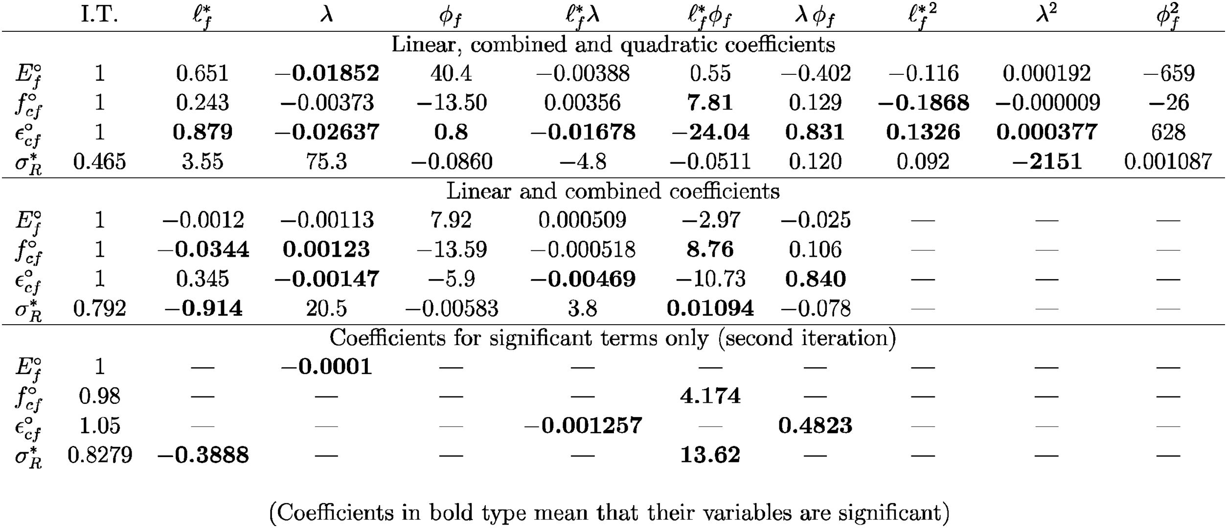
The coefficients obtained for each desired parameter are set forth in Fig. 3. For example, the full response (linear, combined and quadratic) for the compressive strength is:

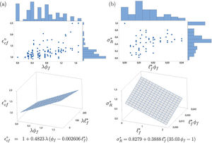
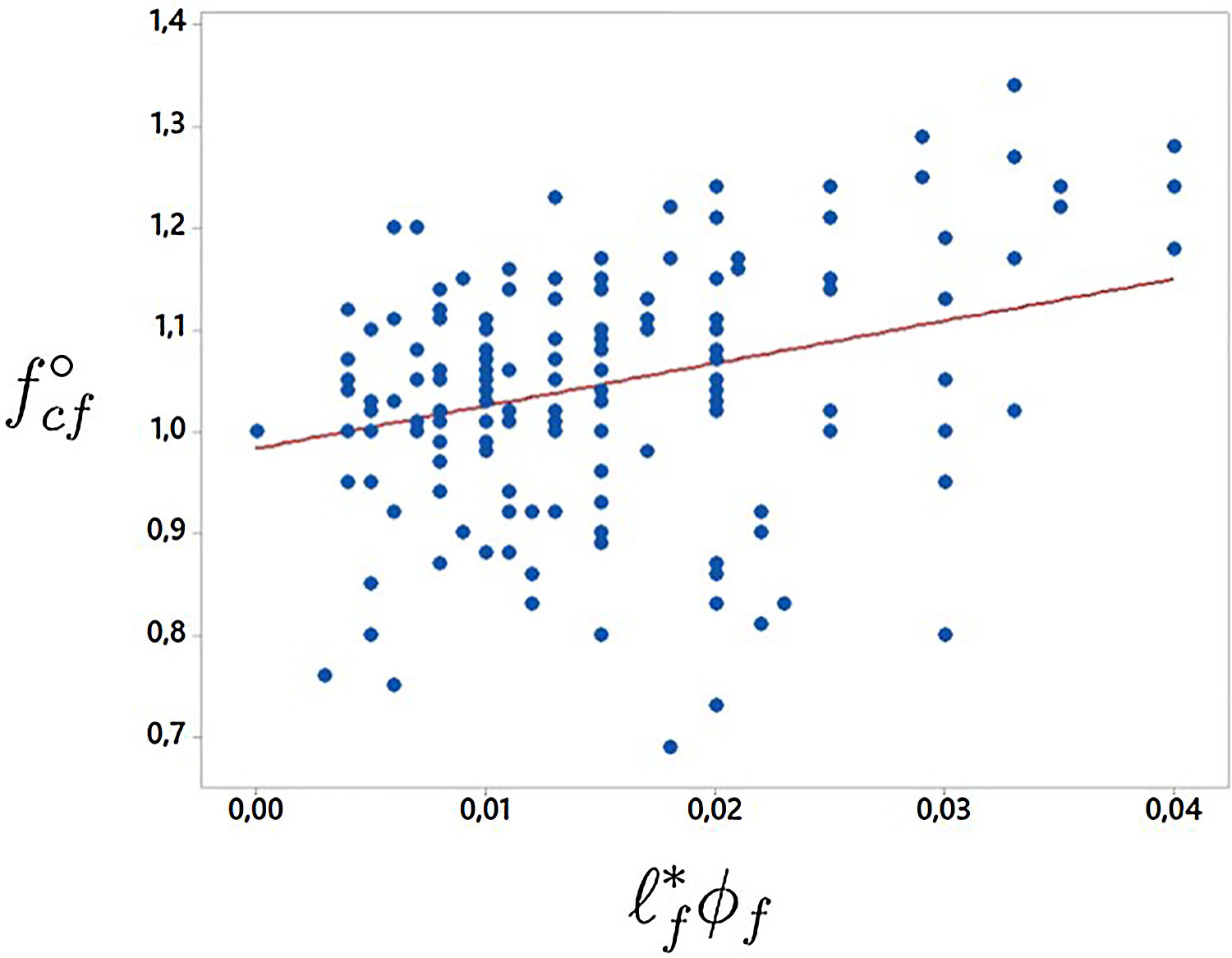
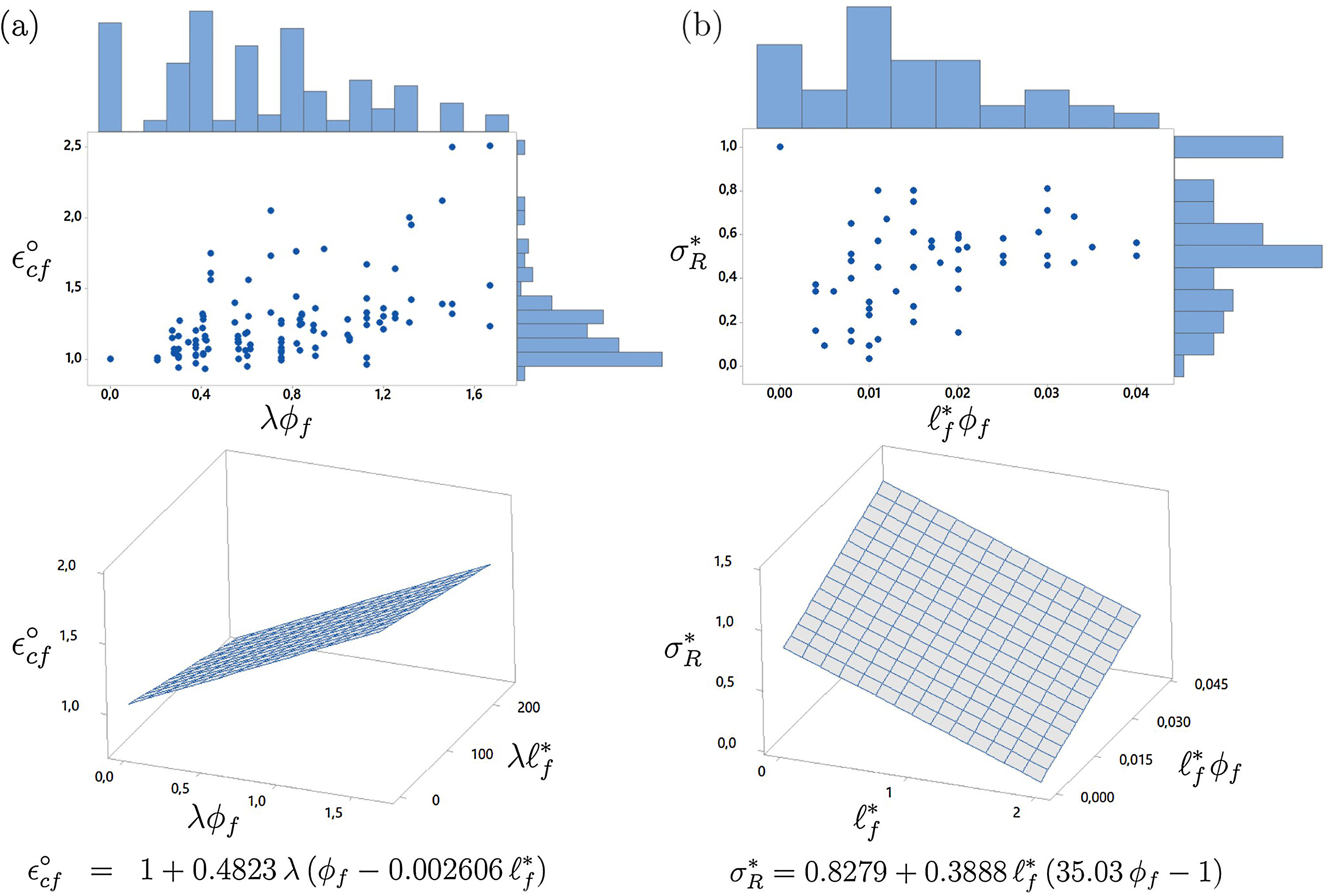
where only the terms corresponding to ℓf*ϕf and to ℓf∗2 are actually significant (this is the reason that their coefficients are written in bold type in Fig. 3). Likewise, we also obtained coefficients for the linear plus the combined response, see Fig. 3. Note that this time we determine that ℓf∗ and λ are significant. In order to derive simpler equations where only significant terms are present, we resort to the correlation again in linear mode and only with terms that had already been found to be significant. The outcome often reveals that some terms were not really significant and, in these cases, we eliminate them and resort to the correlation again. This is how we reach the simplest equation for the parameter under study, in this case, the compressive strength:

Figure 3.

Coefficients for functions to fit the database (I.T. refers to an independent term).

Note that we rounded the independent term to 1, since the methodology does not perform any type of asymptotic study but just simple correlation. The procedure to obtain the remaining responses is similar to the one previously described. Fig. 4 plots Eq. (11) superimposed over the values in the database. It is clear that there is a remarkable dispersion, since fcf mostly correlates with the compressive strength of the base concrete fc0, which is the value chosen to get non-dimensional fcf. This is the reason for which we recommend that fcf and εcf are actually measured, since Eq. (11) is only a rough approximation of the average behavior of tests in the database. Similarly, Fig. 5 plots the database values for εcf and σR as functions of some of the influential non-dimensional parameters in Eqs. (3) and (6), namely λϕf and ℓf*ϕf. It also plots the response surfaces that correspond to these equations. Note that the database values for εcf and σR show less scatter than for fcf.

Figure 4.

Non-dimensional compressive strength f_cf⁰ = (f_cf/f_c0) as a function of parameter ℓf*ϕf   (=ℓfϕf / ℓ0) compared with the experimental values in the database.

Figure 5.

Database values and 3D plots of the selected functions for the non-dimensional (a) critical strain εcf0(=εcf / εc0); and (b) stress corresponding to ε=3 εcf, σR*(=σR / fcf).

Despite having tried to simplify the equations by increasing the average significance of the terms, all the response levels could be used. The response is more accurate indeed when the more complex equations are considered. On the other hand, as already commented above, we did not find a good correlation for the relative elastic modulus (the significance of λ for Efo is very weak, see the Table in Fig. 3). The methodology reveals that fiber content in low dosages does not influence the SFRC compressive response at small strains. We did not propose a type of phase-rule, i.e. such as Ef=E0(1−ϕf)+Esϕf because the database does not find ϕf significant.

5

Conclusions

This technical note proposes a σ–ɛ curve for steel fiber-reinforced concrete (SFRC) in compression, intended for non-linear calculations. The model is described technologically, similarly to that used in structural codes. The model has two distinct stretches. The first describes the σ–ɛ behavior up to the maximum load, following the same curve proposed by Eurocode 2 [21] for plain concrete, but using non-dimensional variables referring to fiber reinforced concrete.

The second stretch is defined as a vertical parabola the vertex of which corresponds to compressive strength. It is must pass through point σR−3εcf, which in turn is estimated by correlation to an extensive database of actual σ–ɛ curves. The correlation to get σR is made so that the average energy below the σ–ɛ curve between εcf and 3εcf in the database equals that of the parabola for the same stretch. Therefore, this assumption for the second part of the σ–ɛ curve yields the same mean energy consumption as tests in the database up to 3εcf. Beyond this point we still use the parabola, which is relatively safe since most of the tests in the database exhibit long tails. The technical note also provides estimates for the compressive strength of the steel fiber-reinforced concrete and for the corresponding critical strain. All the formulas are derived by using the response-surface methodology and a database formed by 197 tests on SFRC (only standard cylinders of SFRC with hook-ended fibers with only one bend).

Regarding the total energy consumption of SFRC in compression, the proposed model reflects that it is approximately four times higher on average than the corresponding energy of the base plain concrete (considering only the energy up to 3 εcf). Therefore, the proposed σ−ε curve can considerably improve the modeling of ductility in SFRC structures.

6

Dedication

This work is dedicated to Dr. Carmen Andrade both for her extensive and deep contribution to research in the field of construction technology and for her leading personal example and friendship.

Acknowledgements

Funding from the Ministerio de Economía y Competitividad through project BIA2015-68678-C2-1-R and International Campus of Excellence CYTEMA is gratefully acknowledged. Ángel de la Rosa expresses his gratitude for the fellowship FPI BES-2016-077458.