Comparing the Intercept Mixture Model with the Slack-Variable Mixture Model

Abstract

Mixture experiments are experiments performed using ingredients whose proportions are restricted. This restriction may result in extremely small range in terms of the mixtures, causing difficulties in model fitting arising from ill-conditioning. The choice of model form is a very important factor in the numerical stability of the information matrix. In this paper, the intercept model is compared against the slack-variable model for mixture experiments. We analyzed if it matter which component is replaced for the constant term in the intercept model, in the sense on numerical stability. We also show by numerical examples that the Correlation Criterion, presented in Kang et al. (2015), does not work for the intercept model. Next, as suggested in the literature, we use linear transformation to alleviate the numerical instability. In addition, we try four transformation methods and choose the best one for the intercept model and the slack-variable model. Finally, we compare the intercept model with the slack-variable model based mainly on the prediction accuracy and numerical stability.

Resumen

Los diseños de experimentos para mezclas son diseños que se llevan a cabo usando ingredientes cuyas proporciones están sujetas a restricciones. Dichas restricciones pueden dar como resultado un rango extremadamente pequeño en términos de las mezclas, causando dificultades en el ajuste del modelo debido a problemas de coli- nealidad. La elección de la forma del modelo es un factor importante en la estabilidad numérica de la matriz de información. En este artículo, se compara el modelo intercepto contra el modelo de variable de holgura en experimentos para mezclas. Se analizó la importancia de cuál componente se remplaza por el término constante en el modelo intercepto, en el sentido de estabilidad numérica. Asimismo, se muestra mediante ejemplos numéricos que el Criterio de Correlación, presentado por Kang et al. (2015), no funciona para el modelo intercepto. Después, como se sugiere en la literatura, se emplearon transformaciones numéricas para mejorar la inestabilidad numérica. Adicionalmente, se probaron cuatro métodos de transformación y se seleccionó el mejor, tanto para el modelo intercepto como para el modelo de variable de holgura. Finalmente, se comparó el modelo intercepto contra el modelo de variable de holgura basado principalmente en la precisión de predicción y la estabilidad numérica.

Introduction

A mixture experiment is one in which the response depends only on the relative proportions of the ingredients, or components, present in the mixture, this proportions represent the design variables. In such experiments, by mixing different components, the product is developed. Mixture experiments frequently appear in fields such as chemical, pharmaceutical, food and plastic industries. There are certain type of mixture experiments where the total amount of the mixture, or process variables, are involve too as a design variables (Piepel and Cornell, 1985; Goldfarb et al., 2004). In this paper, we focus on the mixture experiments with the proportions of the components as the only input variables.

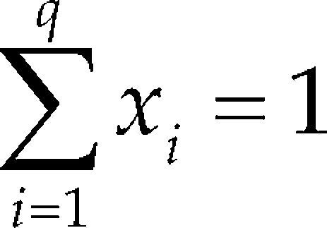
If x_i denotes the proportion of the ith of q components, then xi ≥ 0 for i = 1, 2, ..., q, and

Commonly the design region (1) is subject to additional constraints of the form

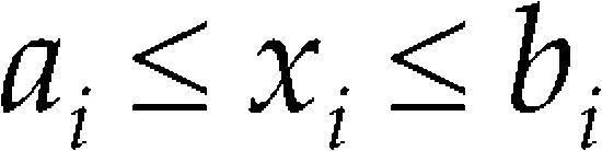
to one or several components. These additional restrictions may result in extremely small range in terms of the mixtures. Not only does the experimental design region become constrained, but the resulting model from a mixture experiment also has to satisfy the constraint. This can cause difficulties in model fitting arising from ill-conditioning. That is, the columns of the corresponding model matrix can be almost linearly dependent (Prescott et al., 2002). Some consequences of ill-conditioning are that the least squares estimators of the parameters have large standard errors and are highly correlated, and the estimates are highly dependent on the precise location of the design points.

Data from a mixture experiment are usually modelled using Scheffé¿s polynomial models (Sheffé, 1958). The quadratic Scheffé¿s model has the general form:

Scheffé¿s model

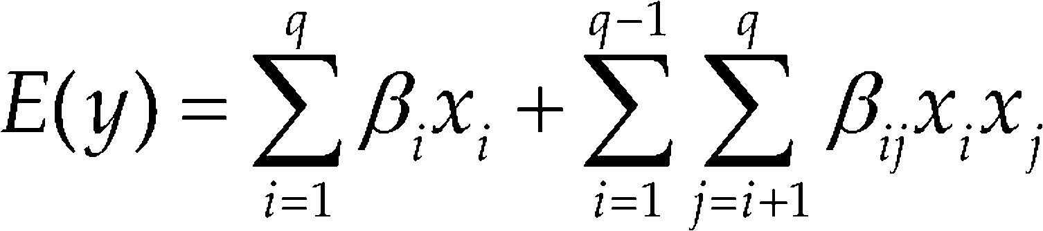
where β_i and β_ij are unknown parameters to be estimated.

Because of the mixture constraint Eq. (1), the quadratic form of Scheffé¿s model involves linear terms and cross-product terms only, but this could be re-parameterized to include square terms (Philip and Norman, 2009). In fact, there are a number of different ways of writing a polynomial model, of any specified order, obtained by re-parameterization using the mixture constraint (Prescott et al., 2002).

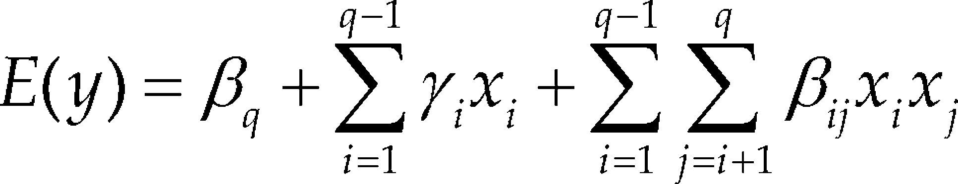
Alternative polynomial model forms include the intercept models, which are obtained by replacing one mixture component, for example x_q, for a constant term. A related model is the slack-variable model, in which one variable (designated the slack variable) is entirely eliminated by substitution; that is, by expressing it in terms of the remaining k – 1 components using Eq. (1), then substituting it into Scheffé¿s model (Piepel and Cornell, 1985). The different between the intercept model and the slack-variable model, is that the slack-variable model has quadratic model terms, while intercept model only present linear and interactions model terms, see (Cornell, 2000; Philip and Norman, 2009; André, 2005). Such re-parameterized models are equivalent in the sense that they lead to the same predicted values and basic analysis of variance (Philip and Norman, 2009). These two models are re-parameterizations of one another and all lead to the same fitted response contours and residuals. The equations may be expressed as follows, with the same symbols being used for parameters that are common to the different models:

Intercept mode

Slack-variable model

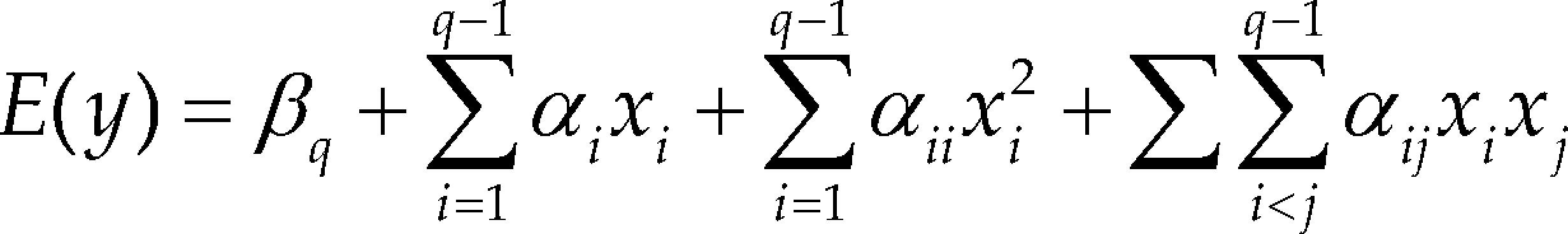
Moreover γ_i = β_i − β_q, α_i = β_i − β_q + β_iq, α_ii = −β_iq and α_ij = β_ij − (β_iq + β_jq).

The pros and cons of the use of intercept models or slack-variable models, as opposed to Scheffé¿s model, have generated a lot of discussions among research workers and practitioners (André, 2005). This issue was discussed by Cornell (2000), one of the questions raised by him was “does it matter which component is designated the slack variable?” He attempted to answer this question by discussing three numerical examples. In André (2005), the same issue was revisited from a different perspective. Emphasis was placed on model equivalence through the use of the column spaces of the matrices associated with the fitted models. It was shown that for the Scheffé¿s complete model and its corresponding slack-variable models, their reduced models, or submodels, provide different types of information. For some reduced models of a given size, Scheffé’s model may provide the best fit, but for other reduced models, some slack-variable models may be preferred. Prescott et al. (2002) propose an alternative pseudo-component-type transformation that leads to model coefficients that represent predictions at a wider selection of points within the design space. This delivers model coefficients that have a much more meaningful interpretation. Prescott and Draper (2002) compare the Scheffé model, the Kronecker model and the intercept model. Recently, Kang et al. (2015) propose a new criterion named “Correlation criterion”, to choose the best Slack-variable model using different components as slack variables, this criterion is only based on the design of the mixture.

In this paper, we analyzed if it matter which component is replaced for the constant term in the intercept model, in the sense on numerical stability. We also show by numerical examples that the Correlation Criterion, presented in Kang et al. (2015), does not work for the intercept model. Next, as suggested in the literature, we use linear transformation to alleviate the numerical instability. In addition, we try four transformation methods and choose the best one for the intercept model and the slack-variable model. Finally, we compare the intercept model with the slack-variable model based mainly on the prediction accuracy and numerical stability.

Method

Diagnostic measures

Below we briefly explain some diagnostic measures that help to detect or identify collinearity (Cornell, 2003; Montgomery and Voth, 1994; Prescott et al., 2002).

Multiple correlation coefficient

We define x_j as the j_th column of X and X_j as the matrix that results when the column x_j is deleted from X. Then Rj2 is the multiple correlation coefficient obtained by regressing x_j on X_j. When the first column of X is a constant column, Rj2 is usually calculated, for j= 2, ..., p, as

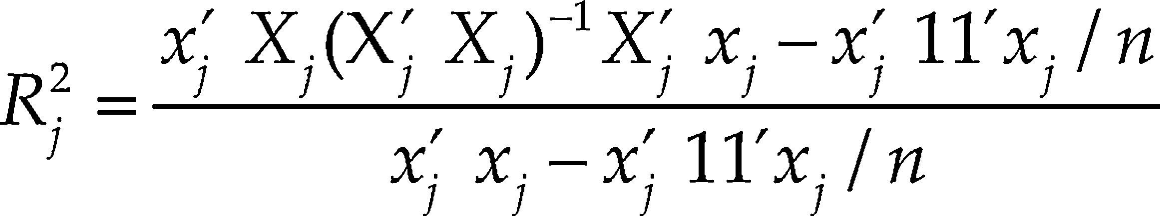
Where 1 is a column of unit elements.

When the column of constants of the X matrix is not available, the unadjusted multiple correlation coefficient can be obtained by

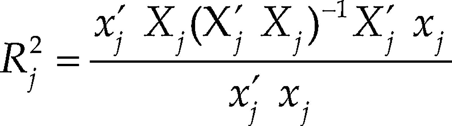
For j = 1, ..., p.

Variance inflation factor

The variance inflation factor (VIF) associated with the estimated regression coefficients β_j is given by

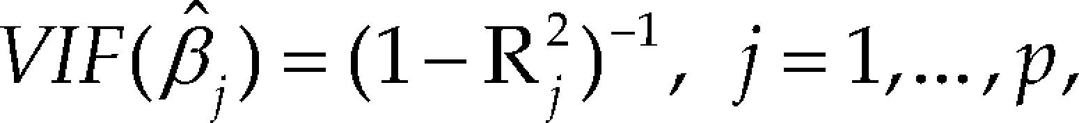
Small values of VIF are an indication of conditioning.

To evaluate the overall collinearity level of a model, it is propose the mean variance inflation factor (MVIF)

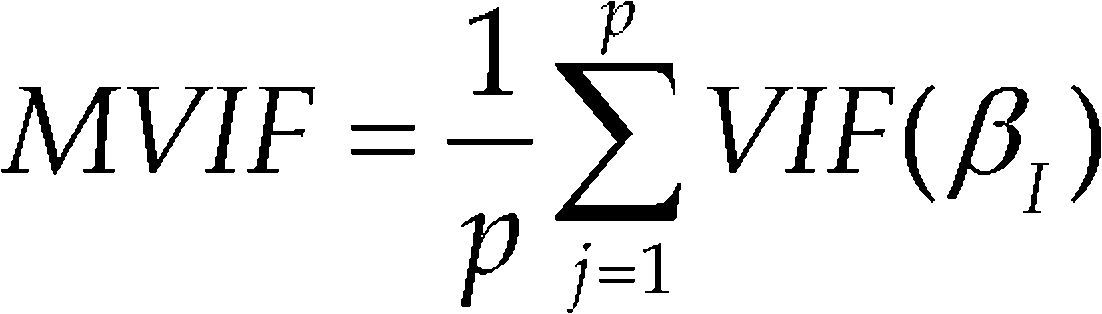
where p is the number of effects in the model, excluding the intercept.

Condition number

Allow λ_max> λ₂ > ... > λ_p−1 > λ_min to be the p eigenvalue of X’ X, which are p solutions to the determinant equation

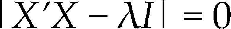
which is a polynomial with p roots.

There are many definitions of the condition number (CN) of a matrix. The general definition used in applied statistics is the square root of the ratio of the maximum to the minimum eigenvalues of X’ X denoted by

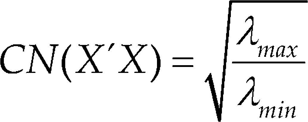
Small values of λ_min and large values of λ^max indicate the presence of collinearity. Low values of the CN indicate some level of stability or conditioning in the least squares estimate.

Remedial measures

Linear transformation is suggested in the literature to alleviate the numerical instability. Below we briefly explain tree linear transformation.

L-Pseudocomponents

When ingredients proportions x_i are restricted by lower bounds L_i while retaining an upper bound of 1, (Kurotori, 1966) recommended using L-pseudocomponents of the form

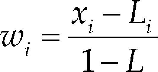
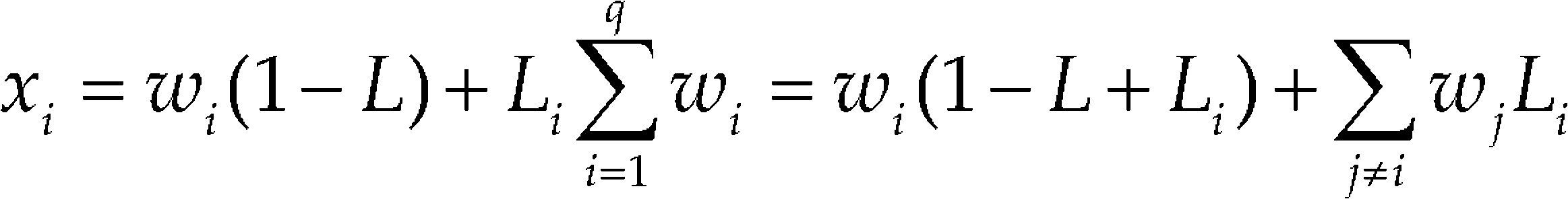
Where L = ∑ L_i. For the restricted mixture space to exist within the simplex, it is necessary that L < 1. Using the Eq. (10) in the pseudocomponent space, we have

for i = 1, ..., q (Prescott et al., 2002).

U-Pseudocomponents

When the range of each ingredient proportion x_i is restricted by an upper bound U_i only, Crosier (1984) recommended the use of U-pseudocomponents, defined as

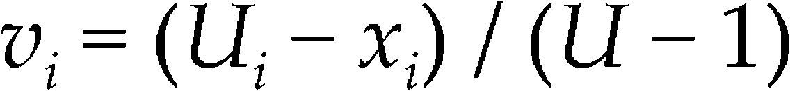
where U = ∑U_i. For the U-simplex to be a region fully within the original simplex, it is necessary that U − 1 ≤U_min (Crosier, 1984). If is requirement holds, then the pseudocomponent transformation

gives only positive multipliers of v_i.

When U − 1 > U_min, the U-simplex extend outside the original mixture simplex and better conditioning may or may not be achieved with U-pseudocomponents, depending on the particular restrictions and the design points.

Modified L-pseudocomponents

For the modified L-pseudocomponent we have to calculate the average over the N observations, x¯l=∑/N, where ∑x¯=1. Next, we calculate the differences x¯l−Li,i=1,2,…,q Suppose the k^th component has the mini- mum difference dk=x¯k−Lk≤di=x¯l−Li,i≠k. Then, instead of all the components being transformed to the L-pseudocomponents as in (10), we use the average of the q − 1 components x_ii ≠ k to define the modified L-pseudocomponents

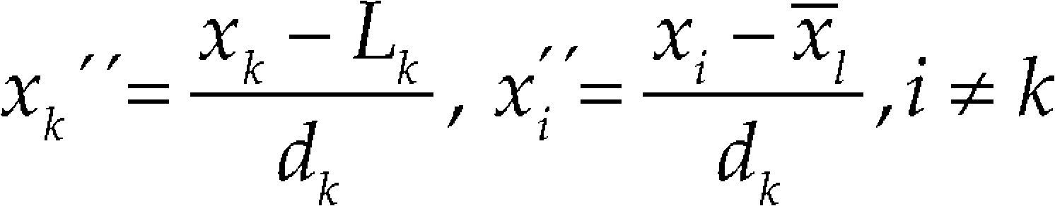
where

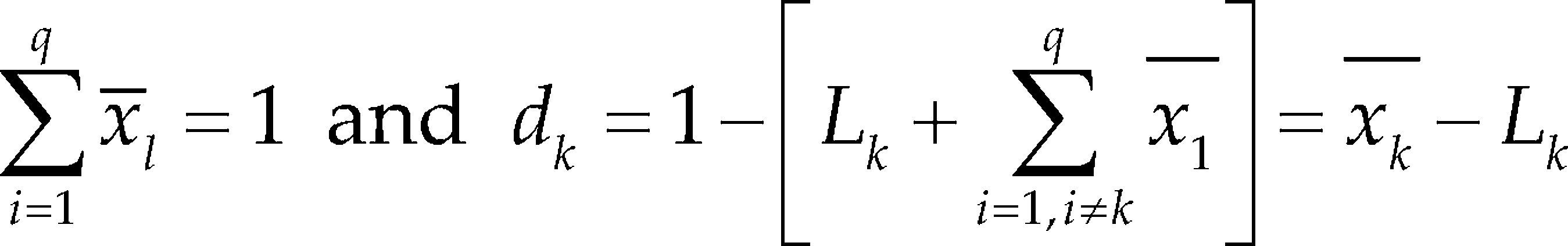
Is a scale constant (Philip and Norman, 2009).

Correlation criterion

Kang et al. (2015) propose a new criterion named “Correlation criterion”, to choose the best Slack-variable model using different components as slack variables. Below we present de Correlation criterion.

Denote F as the design matrix for the mixture experiment of total q components and n experimental settings. Define r_ij as the correlation between the ith and jth columns of F. This correlation is given by

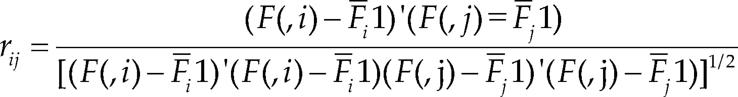
where F (,i) is the ith column of F, F¯i is the sample mean of F (, i), and 1 is a vector of 1's. To evaluate whether the ith column is collinear with any other columns, we can use its average squared correlation with all the q − 1 columns. Denote it as ri2 and it can be calculated by

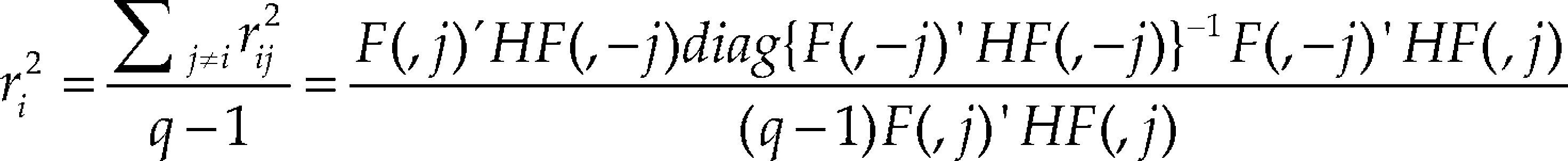
The matrix H is H = I − 1/n 11’and I is the n ⨯ n identity matrix. Thus, we choose the component that has the largest ri2as the slack variable (Kang et al., 2015).

Results and discussion

Four examples to evaluate de correlation criterion in the intercept model

In this section, we compute the correlation criterion in four examples chosen from the literature.

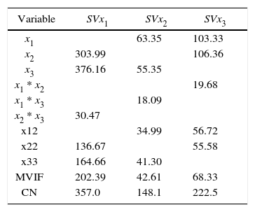
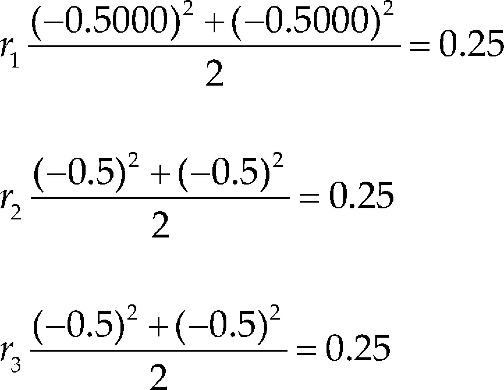
Example 1

We consider the example used by Cornell and Gorman (2009) involving three components and seven design points in the reduced region constrained by the inequalities

Foremost, we compute the correlation criterion. The calculations are presented below

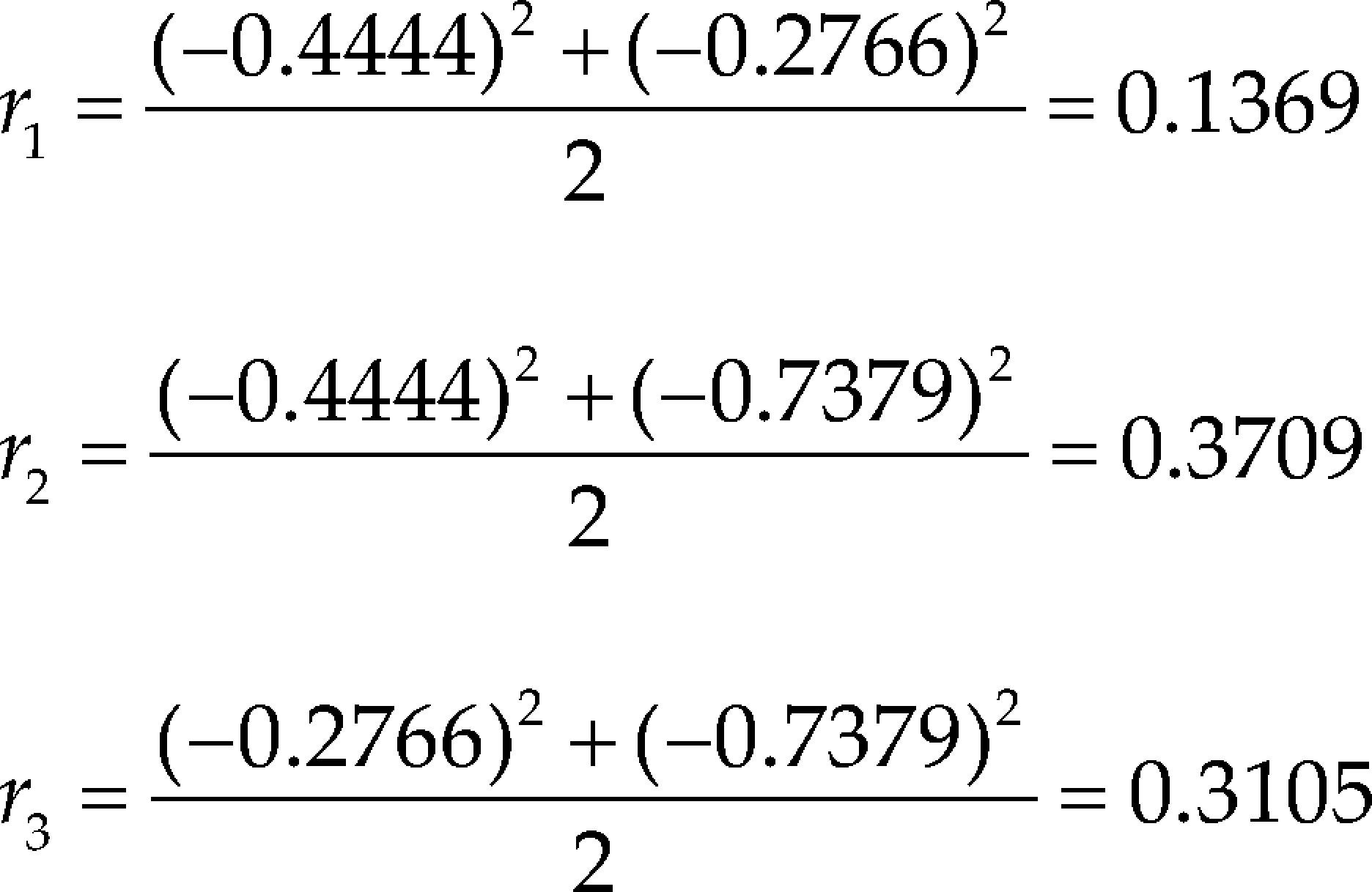
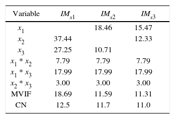
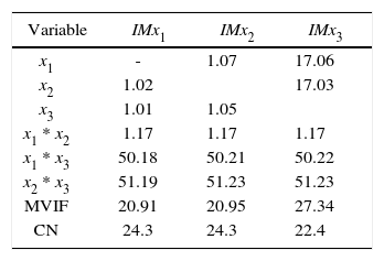
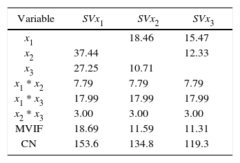
According to the correlation criterion x₂ should be replaced by a constant term. In Table 1 and Table 2 we present the VIF associated with the estimated regression coefficients, MVIF and CN for the three intercept models and the three slack-variable models respectively. We use the expression IM_xi to represent the intercept model replacing x_i for a constant term and SV_xi to represent the slack-variable model using x_i as a slack variable. It can be seen in Table 1 that replacing the component with the largest correlation by a constant term, the most stable intercept model is not achieved. On the other hand, it can be seen in Table 2 that choosing the component with the largest correlation criterion as slack variable, the most stable slack-variable model is achieved.

Table 1.

VIFs, MVIF and CN for IM_Xi Example 1 with original scale.

Variable	IMx1	IMx2	IMx3
x1		18.46	15.47
x2	37.44		12.33
x3	27.25	10.71
x1 * x2	7.79	7.79	7.79
x1 * x3	17.99	17.99	17.99
x2 * x3	3.00	3.00	3.00
MVIF	18.69	11.59	11.31
CN	12.5	11.7	11.0

Table 2.

VIFs, MVIF and CN for SV_Xi Example 1 with original scale.

Variable	SVx1	SVx2	SVx3
x1		63.35	103.33
x2	303.99		106.36
x3	376.16	55.35
x1 * x2			19.68
x1 * x3		18.09
x2 * x3	30.47
x12		34.99	56.72
x22	136.67		55.58
x33	164.66	41.30
MVIF	202.40	42.62	68.34
CN	19.0	12.3	15.0

Example 2

Cornell (2000) considered a three-component, mixture experiment example involving the tint strength of house paint blends. A simplex-centroid design was chosen with the simplex centroid replicated three times. In this example, if we proceed to compute the correlation criterion, we going to see that the value of r_i is the same for the three components (see Tables 3 and 4). Thus, in this case the correlation criterion does not help to decide which component should be replaced for the constant term or should be selected as slack-variable.

Table 3.

VIFs, MVIF and CN for IM_Xi Example 2 with original scale.

Variable	IMx1	IMx2	IMx3
x1	-	1.07	17.06
x2	1.02		17.03
x3	1.01	1.05
x1 * x2	1.17	1.17	1.17
x1 * x3	50.18	50.21	50.22
x2 * x3	51.19	51.23	51.23
MVIF	20.91	20.95	27.34
CN	24.3	24.3	22.4

Table 4.

VIFs, MVIF and CN for SV_Xi Example 2 with original scale.

Variable	SVx1	SVx2	SVx3
x1		17.39	17.39
x2	17.39
x3	17.39	17.39	17.39
x1 * x2
x1 * x3		3.63	3.63
x2 * x3	3.63
x12		14.88	14.88
x22	14.88
x33	14.88	14.88	14.88
MVIF	13.63	13.63	13.63
CN	36.8	36.8	36.8

Example 3

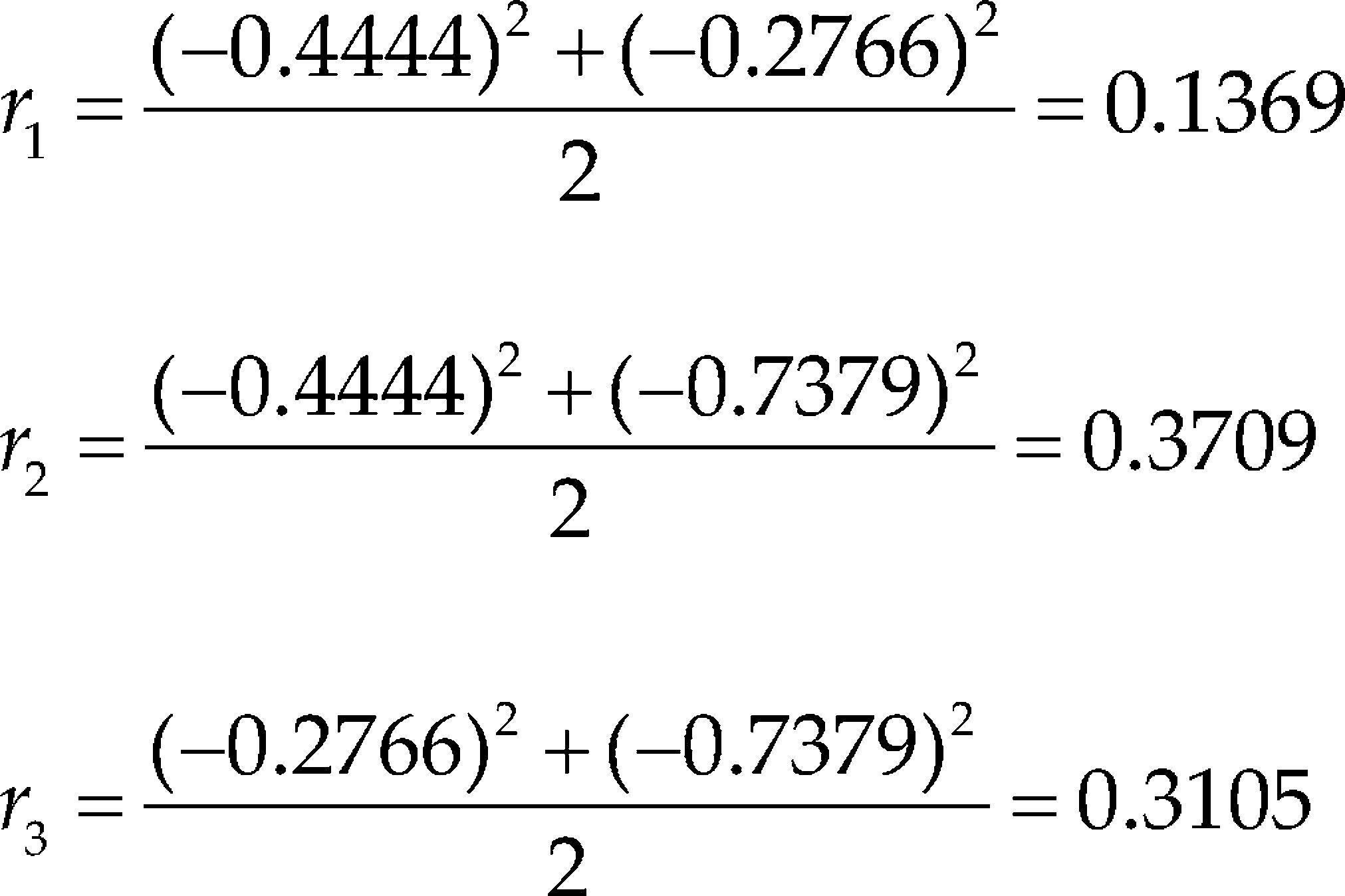
Cornell and Gorman (2003) present a numerical example with three component, ethanol (x₁), water (x₂) and propylene glycol (x₃). Experiment consist in seven-point design. Constraints on the component proportions were: 0.15 ≤ x₁ ≤ 0.50, 0.20 ≤ x₂ ≤ 0.70, 0.15 ≤ x₃ 0.65. As can be seen in Table 5, again the correlation criterion dose not determine the most stable intercept model.

Table 5.

VIFs, MVIF and CN for IM_Xi Example 3 with original scale.

Variable	SVx1	SVx2	SVx3
x1		18.46	15.47
x2	37.44		12.33
x3	27.25	10.71
x1 * x2	7.79	7.79	7.79
x1 * x3	17.99	17.99	17.99
x2 * x3	3.00	3.00	3.00
MVIF	18.69	11.59	11.31
CN	153.6	134.8	119.3

Table 6.

VIFs, MVIF and CN for SV_Xi Example 3 with original scale.

Variable	SVx1	SVx2	SVx3
x1		63.35	103.33
x2	303.99		106.36
x3	376.16	55.35
x1 * x2			19.68
x1 * x3		18.09
x2 * x3	30.47
x12		34.99	56.72
x22	136.67		55.58
x33	164.66	41.30
MVIF	202.39	42.61	68.33
CN	357.0	148.1	222.5

Example 4

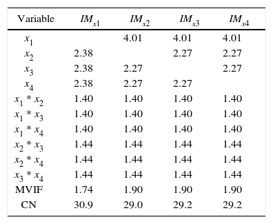
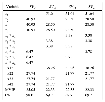
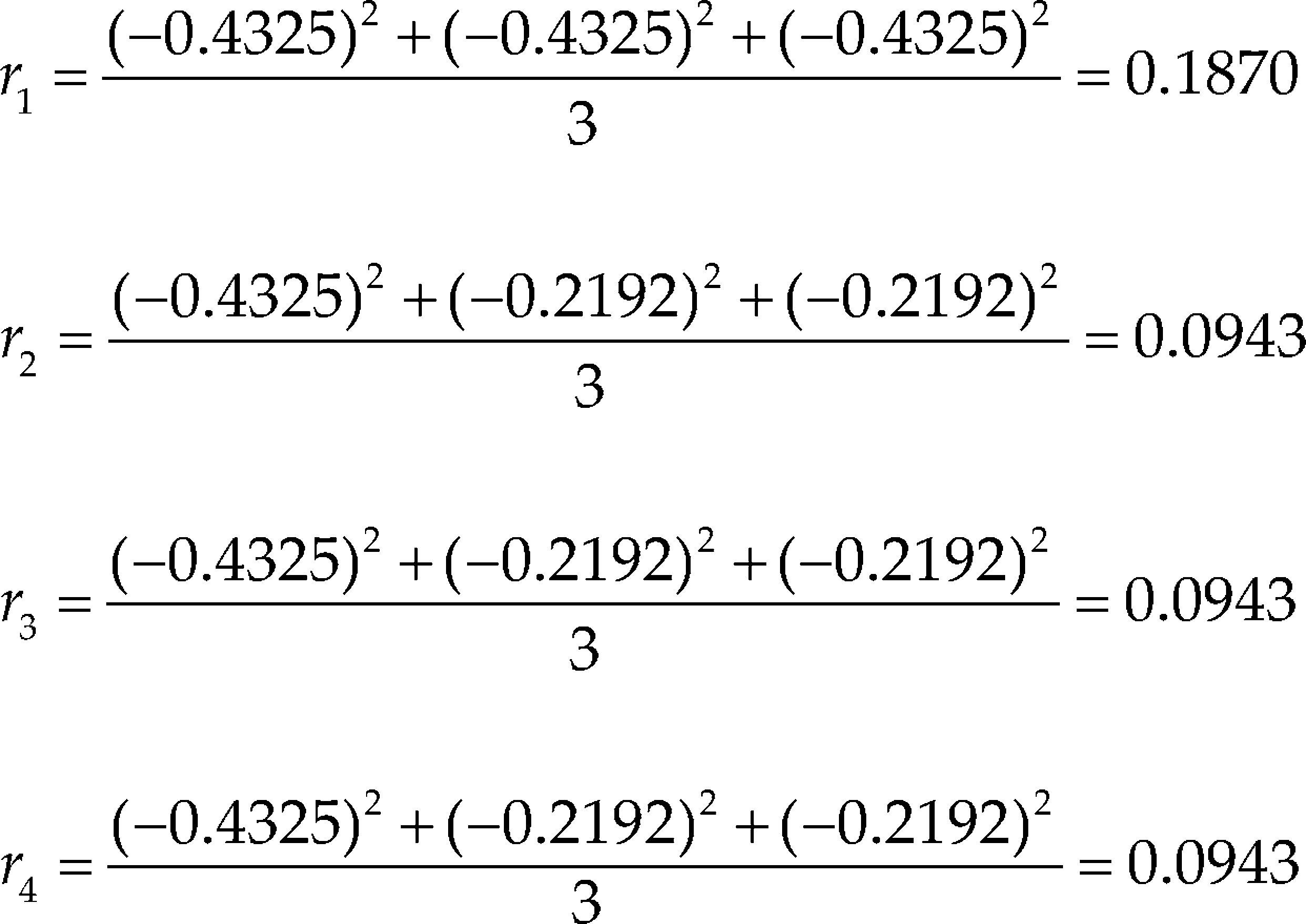
Cornell (2002) present an example named The Formulation of a Tropical Beverage. A tropical beverage was formulated by combining juices of watermelon (x₁), orange (x₂), pineapple (x₃), and grapefruit (x₄). In this example, the component with the largest r_i is x₁, however, as can be seen in Tables 7 and 8, the most stable intercept model is achieved replacing component x₂, and the most stable slack-variable model is achieved using any of the three x₂, x₃ and x₄ components.

Table 7.

VIFs, MVIF and CN for IM_xi Example 4 with original scale.

Variable	IMx1	IMx2	IMx3	IMx4
x1		4.01	4.01	4.01
x2	2.38		2.27	2.27
x3	2.38	2.27		2.27
x4	2.38	2.27	2.27
x1 * x2	1.40	1.40	1.40	1.40
x1 * x3	1.40	1.40	1.40	1.40
x1 * x4	1.40	1.40	1.40	1.40
x2 * x3	1.44	1.44	1.44	1.44
x2 * x4	1.44	1.44	1.44	1.44
x3 * x4	1.44	1.44	1.44	1.44
MVIF	1.74	1.90	1.90	1.90
CN	30.9	29.0	29.2	29.2

Table 8.

VIFs, MVIF and CN for SV_xi Example 4 with original scale.

Variable	SVx1	SVx2	SVx3	SVx4
x1		51.64	51.64	51.64
x2	40.93		28.50	28.50
x3	40.93	28.50		28.50
x4	40.93	28.50	28.50
x1 * x2			3.38	3.38
x1 * x3		3.38		3.38
x1 * x4		3.38	3.38
x2 * x3	6.47			3.78
x2 * x4	6.47		3.78
x3 * x4	6.47
x12		38.26	38.26	38.26
x22	27.74		21.77	21.77
x33	27.74	21.77		21.77
x42	27.74	21.77	21.77
MVIF	25.05	22.33	22.33	22.33
CN	98.0	69.7	69.7	69.7

To summarize this section, we can point out that the intercept model can be used, in order to alleviate the collinearity problem. As could be seen in the examples shown in this section, the choice of which component is replaced for the constant term is crucial in the sense on numerical stability. However, the choice of which component should be replaced for a constant term, cannot be performed according with the correlation criterion. We recommend practitioners directly construct each possible intercept model matrix and choose the best one according to maxVIF, MVIF and CN criterion.

Linear transformations

To analyze mixture experiments, it is suggested to perform some linear transformation on the components’ proportions to reduce the ill-conditioning problem. However, different transformation methods work the best for different mixture models. For the slack-variable model, Kang et al. (2015) recommend scale the design of the proportion into [–1, 1], which is the typical scale used in classical design and analysis of experiments. For other mixture models L–, U– and modified-pseudocomponent transformations are recommended for the literature. Thus, we try all four transformation methods and choose the best one for the intercept model and the slack-variable model.

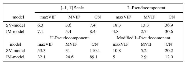
Example 5

In this example, we used the Example 1 data (Cornell and Gorman, 2009) and applied the four transformation, in order to choose the best one according to maxVIF, MVIF and CN. Based on Table 9, for this example, scaling the components’ proportions into [–1, 1] range works the best for the two models. In this case, the slack-variable model is the most parsimonious model.

Table 9.

Comparison of the complete IM model and SV model using the Example 1 data, with different transformation.

	[–1, 1] Scale			L-Pseudocomponent
model	maxVIF	MVIF	CN	maxVIF	MVIF	CN
SV-model	6.3	3.6	7.4	18.3	13.3	36.9
IM-model	7.1	5.4	8.4	4.8	2.7	30.6
	U-Pseudocomponent			Modified L-Pseudocomonent
model	maxVIF	MVIF	CN	maxVIF	MVIF	CN
SV-model	53.3	31	110.1	10.8	5.2	20.2
IM-model	32.1	24.6	89.1	5	2.9	12.0

Example 6

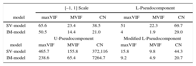
For the Example 6, we used the Example 4 data (Cornell, 2002) and applied the four transformation, in order to choose the best one according to maxVIF, MVIF and CN. Based on Table 10, for this example, the modified L– Pseudocomponent transformation works the best for the intercept model while scaling the components’ proportions into [–1, 1] range works the best for the slack-variable model. In this case, the intercept model is the most parsimonious model.

Table 10.

Comparison of the complete IM model and SV model using the Example 4 data, with different transformation.

	[–1, 1] Scale			L-Pseudocomponent
model	maxVIF	MVIF	CN	maxVIF	MVIF	CN
SV-model	65.6	23.4	38.5	51	22.3	69.7
IM-model	50.5	14.4	21.0	4	1.9	29.0
	U-Pseudocomponent			Modified L-Pseudocomponent
model	maxVIF	MVIF	CN	maxVIF	MVIF	CN
SV-model	465.7	155.8	372,116	15.8	9.8	44.3
IM-model	238.6	65.4	7264.7	9.2	4.9	20.7

Numerical stability and prediction accuracy comparison

The choice of model forms can affect the numerical stability of the information matrix. In this section, we compare the intercept model with the slack-variable model based mainly on the prediction accuracy and numerical stability.

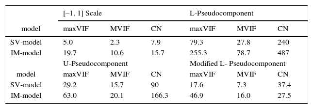
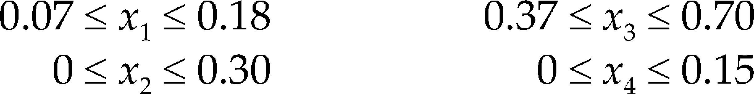
Example 7

In this section, we use the example presents in John (1984), the experiment involves an additive x₁ and three lubricant blends x₂, x₄ and x₄. The component proportions need to satisfy

First, we use different transformation methods for the two models and choose the best one according to maxVIF, MVIF and CN in Table 11. According to Table 11 scaling the components’ proportions into [–1, 1] range works the best for both models. In this case, the slack-variable model is the most parsimonious model.

Table 11.

Comparison of the complete IM model and SV model using the Example 7 data, with different transformation.

	[–1, 1] Scale			L-Pseudocomponent
model	maxVIF	MVIF	CN	maxVIF	MVIF	CN
SV-model	5.0	2.3	7.9	79.3	27.8	240
IM-model	19.7	10.6	15.7	255.3	78.7	487
	U-Pseudocomponent			Modified L- Pseudocomponent
model	maxVIF	MVIF	CN	maxVIF	MVIF	CN
SV-model	29.2	15.7	90	17.6	7.3	37.4
IM-model	63.0	20.1	166.3	46.9	16.0	27.5

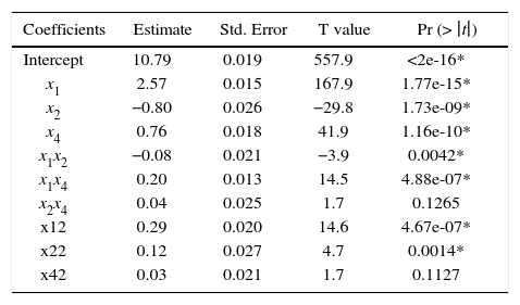
In Table 12 we present the analysis of variance (ANOVA) for the slack-variable model using Example 7 date and scaling the components’ proportions into [–1, 1] range. As can be seen in Table 12, the interaction x₂, x₄ and the quadratic term x42 have no statistical significance effect over the response according with de P-value at 99% confidence level. Thus, both terms can be removed from the model.

Table 12.

ANOVA for the Slack-variable model into [–1, 1] range. Significant codes 0.01 “*”.

Coefficients	Estimate	Std. Error	T value	Pr (> ∣t∣)
Intercept	10.79	0.019	557.9	<2e-16*
x1	2.57	0.015	167.9	1.77e-15*
x2	−0.80	0.026	−29.8	1.73e-09*
x4	0.76	0.018	41.9	1.16e-10*
x1x2	−0.08	0.021	−3.9	0.0042*
x1x4	0.20	0.013	14.5	4.88e-07*
x2x4	0.04	0.025	1.7	0.1265
x12	0.29	0.020	14.6	4.67e-07*
x22	0.12	0.027	4.7	0.0014*
x42	0.03	0.021	1.7	0.1127

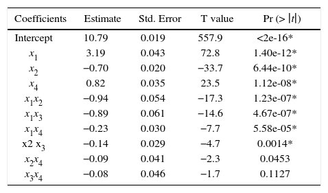
On the other hand, in Table 13 we present the ANOVA for the intercept model using Example 7 date and scaling the components’ proportions into [–1, 1] range. As can be seen in Table 13, the intercept terms x₂, x₄ and x₃, x₄ have no statistical significance effect over the response according with P-value at 99% confidence level. Thus, again we can removed both terms from the model.

Table 13.

ANOVA for the Intercept model into [–1, 1] range. Significant codes 0.01 “*”.

Coefficients	Estimate	Std. Error	T value	Pr (> ∣t∣)
Intercept	10.79	0.019	557.9	<2e-16*
x1	3.19	0.043	72.8	1.40e-12*
x2	−0.70	0.020	−33.7	6.44e-10*
x4	0.82	0.035	23.5	1.12e-08*
x1x2	−0.94	0.054	−17.3	1.23e-07*
x1x3	−0.89	0.061	−14.6	4.67e-07*
x1x4	−0.23	0.030	−7.7	5.58e-05*
x2 x3	−0.14	0.029	−4.7	0.0014*
x2x4	−0.09	0.041	−2.3	0.0453
x3x4	−0.08	0.046	−1.7	0.1127

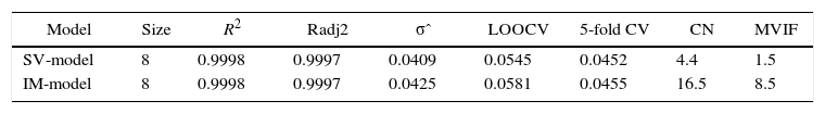
Table 14 shows the comparison of the reduced slack variable model and the intercept model.

Table 14.

Comparison of the reduced intercept model and slack-variable model into [–1, 1] range.

Model	Size	R^2	Radj2	σˆ	LOOCV	5-fold CV	CN	MVIF
SV-model	8	0.9998	0.9997	0.0409	0.0545	0.0452	4.4	1.5
IM-model	8	0.9998	0.9997	0.0425	0.0581	0.0455	16.5	8.5

R² and Radj2 are the coefficient of determinant and the adjusted version, and σˆ is MSE from the ANOVA. LOOCV and 13-fold CV are the leave-one-out and 13-fold cross validation prediction errors. Both reduced models have 8 terms including the intercept and the same fit quality. Table 14 show that slack-variable model present the best prediction accuracy and the most parsimonious model in terms of numerical stability.

Conclusion

In this paper, we analyzed if it matter which component is replaced for the constant term, in the intercept model, in the sense on numerical stability. By numerical examples, in section: Four examples to evaluate de correlation criterion in the intercept model we showed that the intercept model can be used to reduce the ill-conditioning problem. In addition, evidence was given that the choice of which component is replaced for the constant term is crucial in the sense on numerical stability. Moreover, we computed the correlation criterion and we determined that this criterion does not work for the intercept model, that is, the choose of which component should be replaced for a constant term, cannot be performed according with the correlation criterion. We recommend practitioners directly construct each possible intercept model matrix and choose the best one according to maxVIF, MVIF and CN criterion.

In section: linear transformations we tried four transformation methods and choose the best one for the intercept model and the slack-variable model. Scaling the components’ proportions into [–1, 1] range works the best for the slack-variable model, the modified L–Pseudocomponent transformation works the best for the intercept model in some cases.

Finally, in section: numerical stability and prediction accuracy comparison we compare the intercept model with the slack-variable model based mainly on the prediction accuracy and numerical stability. The slack-variable model has the best prediction accuracy and is the most parsimonious model in terms of numerical stability.

Acknowledgements

This research was supported by CONACYT, UPB and CIATEC.