Dynamic estimation of an interest rate structure in Colombia. Empirical analysis using the Kalman filter

Abstract

The official estimation for the term structure model in Colombia is based on the Nelson and Siegel (1987) development which is widely accepted and used. This estimation is based on the curve fitting with available data, only for one day ahead, making difficult to estimate the future zero-coupon yield curve. Taking into account the importance of having an estimation of the term structure for the valuation of financial assets in the Colombian market, this research proposes a methodology to estimate in a dynamic form the parameters of interest rates in the Nelson and Siegel Model. This required the use of the re-parameterization proposed by Diebold and Li (2006), which determines the shape of the term structure through latent factors such as level, slope and curvature. This paper aims to show the dynamic estimation of the term structure of interest rate using the Kalman filter methodology framed in State - space. Results show that predictions are successful for more than one period in the future.

Resumen

La estimación oficial para el modelo de estructura de plazos en Colombia se basa en el modelo desarrollado por Nelson y Siegel (1987), ampliamente aceptado y utilizado. Dicha estimación se basa en la curva adecuada a los datos disponibles, únicamente a un día vista, lo que dificulta la estimación de la curva de rendimiento de los cupones cero futuros. Teniendo en cuenta la importancia de disponer de una estimación de la estructura de plazos para la valoración de los activos financieros en el mercado colombiano, esta investigación propone una metodología para estimar, de manera dinámica, los parámetros de los tipos de interés dentro del modelo de Nelson y Siegel. Esto requirió el uso de la reparametrización propuesta por Diebold y Li (2006), que determina la forma de la estructura de los plazos mediante factores latentes tales como nivel, pendiente y curvatura. Este documento trata de mostrar la estimación dinámica de la estructura de plazos de los tipos de interés, utilizando la metodología del filtro de Kalman que se enmarca dentro del espacio del Estado. Los resultados reflejan que las predicciones son exitosas para más de un período a futuro.

1

Introduction

Asset pricing strategies are of extreme importance for portfolio managers whose structures admit fixed assets; therefore, estimation, management and forecasting of the term structure of interest rates of the market, that could be national, industrial or sectorial, in which they operate become essential.

Forecasting, regardless of its nature, is crucial in the investment portfolio management for the achievement of desired results and management of the involved risk. So, having a methodology that permits to forecast the term structure of interest rates, taking into account those models that regulators ask market agents to respect, is of extreme relevance.

As for the Colombian market, the official interest rate model adopted by regulators is the one proposed in 1987 by Charles R. Nelson and Andrew F. Siegel, in order to value the market prices and to construct diverse financial products as well as derivatives connected to the interest rate. This methodology presents benefits such as the simplicity of estimation, generalized use by academicians and practitioners and its adjustment to real interest rates in the market. However, the process of parameter estimation, given that the variables are not dependent upon time, impedes its future estimation and, also its calculation requires to be contrasted with the observed values in the market performance curve.

In 2006, Francis X. Diebold and Canlin Li in their paper “Forecasting the term structure of government bond yields” interpret the parameters of the Nelson and Siegel Model (1987) as latent factors of level, slope and curvature of the term structure of the interest rate. This reparametrization allows using a set of recursive equations as the ones established in the Kalman filter in order to obtain the possible form and future level of the curve of interest rates for Colombia.

This paper is divided in five sections. The first one is this introduction; the second describes the theoretical framework. The third presents the used methodology in the research. The fourth details the obtained results from the model, and finally conclusions are shown.

2

Theoretical framework

Our research goal is centered in the forecasting of the form of the term structure of interest rates for Colombia; the paper focuses on the interest rates and forecasting models.

2.1

Stochastic models

In the field of forecasting models of the term structure, the most recognized works in academic literature are Black, Derman, and Toy (1990), Cox, Ingersoll, and Ross (1985), Oldrich and Vasicek (1977), and Ho and Lee (1986).

The Black, Derman, and Toy (1990) model of short rates assumes a lognormal distribution in order to eliminate possible negative rates. A drawback of this model is the possibility to find a closed-form solution that allows the construction of the tree, which is obtained in the term structure, to be based on the forward rates and the volatility process and, not using a forward induction process. This takes the structure of volatilities as an input, and entails a reversion process to the mean. The assumptions used in the model are: changes in the bonds yields are perfectly correlated, the expected yield is the same for all the assets in the same period, there are no taxes or transaction costs and, the distribution of short rates is lognormal. As a result, this model obtains future short term rates consistent with the term structure used as an input.

Cox, Ingersoll, and Ross (1985) is well known as CIR. This model is based on the scheme of a productive process for an economy in which each individual must decide whether to consume or to invest a limited capital, and money could be loaned. The equilibrium is achieved when the interest rate reaches the point in which no individual could feel the need to borrow money, known as the equilibrium market price. The model explains the movements in the interest rate in terms of individual preferences. The short rate assumes the risk in the productive process of the economy, and this determines the complete term structure and, therefore the valuation of the interest rate contingent claim. The long term must be compensated by a premium. The model entails a reversion process to the mean and, is lognormal given the interest rate volatility is positively related to the interest rate level. The great drawback is that the model does not provide an adequate estimation of the long term structure.

The work of Oldrich and Vasicek (1977) is an equilibrium model in conditions of no arbitrage, through the determination of a parabolic differential equation that characterizes the price of a zero-coupon bond. It is a model in continuous time with reversion to the mean in an efficient market, in which the instantaneous spot rate follows a continuous process of Markov and the price of a discount bond only depends on the spot rate during its established term. The assumptions consider that the variance is constant and shows closed solutions as a result.

Ho and Lee (1986) is a model based on the assumption that the no arbitrage of the interest rate, which does not consider market frictions, transactions costs or taxes, works in a discrete and finite time. Ho and Lee (1986) model the uncertain behavior of the term structure of interest rates through the construction of a binomial tree and, obtain as a result an interest rate structure with a perfect adjustment to the forward rate structure that is used as initial input.

2.2

Nelson and Siegel model (1987)

The Nelson and Siegel model (1987) provides a methodology of parametric estimation of a yield curve that adjusts to the market observations and concentrates in the evolution of the instantaneous forward rate. This is a non-polynomial model that aims to eliminate irregular jumps in the interest rate structure, that is, the theoretical yield curve. The main benefit is its simplicity and, therefore its generalized use by academicians and market practitioners. In the Colombian case, the curve constructed under this model's methodology is used as a reference curve to value fixed assets given market prices, among many other applications.

The model has various assumptions. It concentrates on the evolution of the instantaneous forward rate, which dynamic can be modeled by a second-order ordinary differential equation solution, particularly with equal and real roots. The ordinary differential equation can present different forms: monotone, concave, S-shape, as to mention the most common and it is not an general equilibrium model, which means that has no economic interpretation of the agent behavior in their markets.

Considering that the Nelson and Siegel model solution is reached by a second-order ordinary differential equation solution with equal and real roots, the Nelson and Siegel function for instantaneous forward rates with maturation in t is represented as:

The previous equation can take different forms depending on the parameters’ values. One of those forms that can be observed is the monotone, S-shape or concave. Finally, if the previous forward rate equations is integrated, the spot rate (s(t)) is obtained:

Given that (β0 β1 β2 τ) are the parameters to be estimated in the model:

β0 is the contribution of the long term component, and it never tends to zero.

β1 is the contribution of the short term component, as it increases t rapidly tends to zero.

β2 is the contribution of the midterm component, and increases as t reaches its maximum value and then decays.

τ is the speed that β1 and β2 converge to zero. The inverse 1/τ is the acceleration that the instantaneous forward rate converges in the long term β0.

Given the nature of the model solution, a great drawback is evidenced. The parameters are not dynamic or time dependent, and it is precisely the focus of our empirical work.

2.3

Diebold and Li model (2006)

Diebold and Li interpret the parameters of the Nelson and Siegel model (1987) as factors of level, slope and curvature of the term structure of interest rates. Basically, they have the same viewpoint of Nelson and Siegel (1987) about the second-order ordinary differential equation to obtain the following function for the forward rate.

However, taken the elaborated reparametrization, the function is expressed as follows:

Taking into account that λ=1τ, y  τ=t, if we want to make this equivalent to Nelson and Siegel (1987).

After having knowledge of the forward rates curve of Diebold and Li (2006), the spot rate for a zero-coupon with expiration in Tau can be determined as the weighted average of the forward rates, and in this point we do the following derivation based on the original work.

Alvaro Solera (2003) in his paper written for the Banco Central de Costa Rica (Costa Rican Central Bank), clearly describes the process of filter algorithm,

2.4

Empirical work

The objective of our research is the future estimation or forecasting of the parameters of the Nelson and Siegel model (1987) through the mathematical tools described in the previous section, to finally complete the construction of a dynamic zero-coupon yield curve for the Colombian case.

2.5

Data

For the purpose of this research, it was necessary to account the daily parameters of the Nelson and Siegel model (1987) from May 2^nd, 2003 to February 28^th, 2011, which provides a total of 1973 periods. A term structure was constructed using the aforementioned data, and 20 expirations were determined: 0.25, 0.5, 0.75, 1, 1.25, 1.5, 1.75, 2, 2.5, 3, 4, 5, 6, 7, 8, 9, 10, 11, 12 and 13 years.

This information is available in the webpage of Infoval, a provider of prices, rates and margins for the valuation of Colombian assets. However, these data can be also obtained through the observation of daily negotiated rates of public debt bonds class B – TES, following the valuation methodology by Infoval.

2.6

Proposed model

Following Francis Diebold and Canlin Li (2006) model in which they interpret the Nelson and Siegel model (1987) in terms of three latent factors: level, slope and curvature, for the estimation of a term structure of interest rates; a future estimation of these latent factors through a Kalman filter in order to obtain a possible form and level that the Colombian interest rate curve could have.

Thus, our mathematical model is represented as follows:

In which:

The parameters to estimate through the Kalman filter are β0t,β1t and β2t.

2.7

Estimation from the proposed model

Given that the estimation process has been done through a Kalman filter and Kalman (1960), the first step is to determine each one of the matrices involved in the model.

2.8

Initial estimations

The seed or start-up values of βt−1ˆ and Pt−1 must be defined. Where:

Matrix βt−1ˆ is the matrix of the estimate parameters of the previous period. The scale of this matrix is 3x1. For the start-up period of the forecasting is used as seed the last observed parameters that are available.

Matrix Pt−1 is the same error covariance forecasting of the model, but of the period t-1 to elaborate the forecasting of the next step. Its scale is 3x3 and for the first forecasting period, the seed value can be the one of the Q matrix of the first period.

2.9

Forecasting equations

a) Forecasting of state

In which:

Matrix F is the relation between the parameters to be estimated taking the ones of the previous period. This matrix can have a scale of 3x3. We based our proposal on the fact that the model not only forecasts, but also corrects this matrix that serves as seed datum to forecast as a diagonal matrix. This diagonal has values of 1, taking into account the precept that the best forecast that could be obtained for tomorrow is today's value plus an error.

b) Error covariance forecasting

In which:

Matrix P^*_t is the error covariance forecasting of the model. The scale is 3x3. This matrix is updated as the filter works.

Matrix Q is the value of variances of state error. The scale is 3x3.

2.10

Correction equation

a) Kalman profit

In which:

Matrix H shows the loadings of the latent factors of the Diebold and Li model. Its scale is 20x3, and it is referred to equation (3) in the proposed model.

Matrix R contains the error variances of the observations. Its scale is 20x20.

b) Update of the measure

In which:

Matrix Y_t is the matrix of the model's yield forecasting, to be specific equation (3) of the proposed model. Its scale is 20x1.

c) Error covariance update

In which:

Matrix I is a matrix of identity with a scale of 3x3.

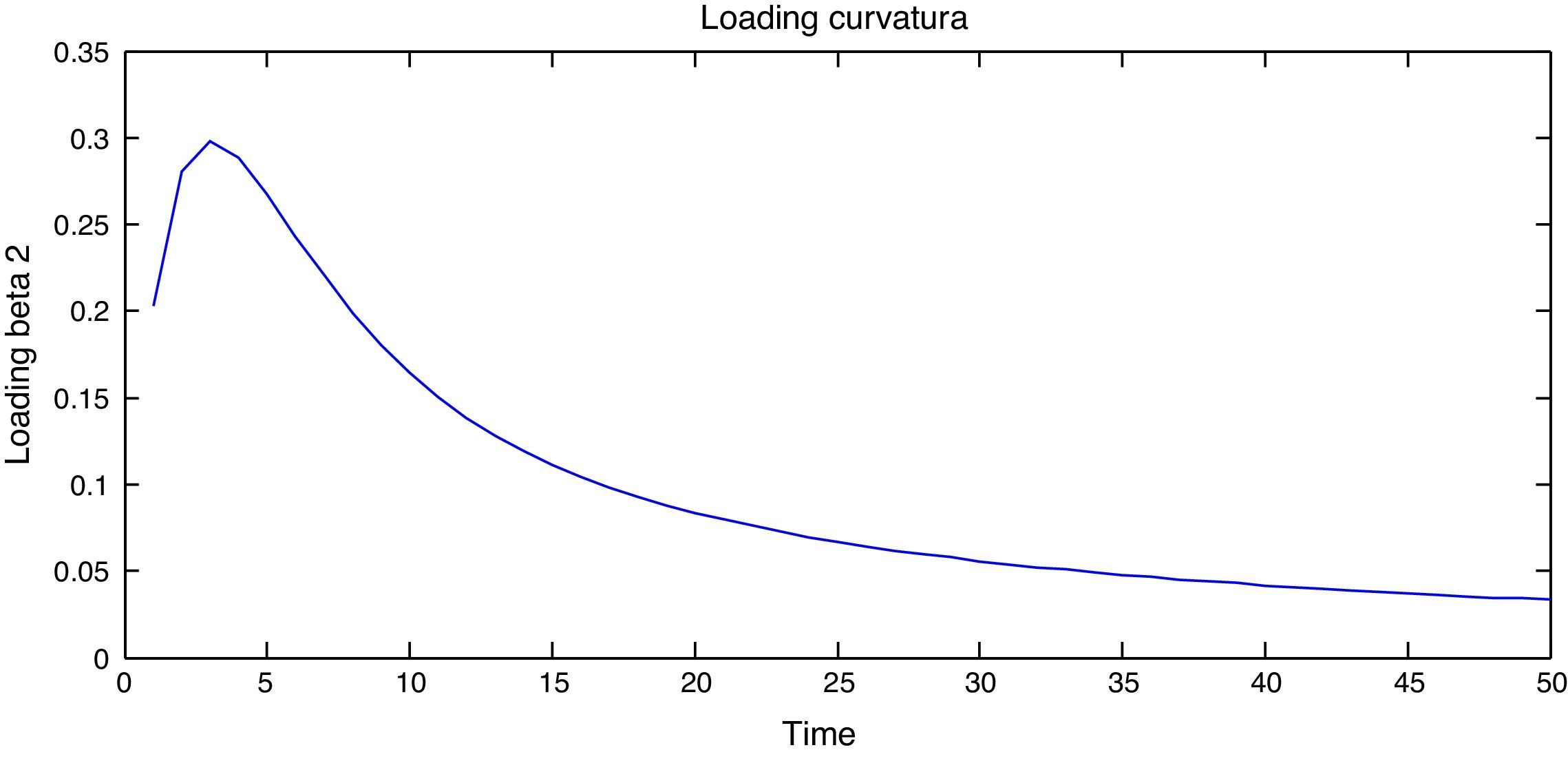
3

Results

Lambda, as it is established by Diebold and Li (2006), should be taken as a constant in order to estimate the other parameters in a lineal estimation. This factor will be the value that maximizes the loading of the factor in the curvature (β_2t) in the period considered adequate for the economy being studied, specifically, the Colombian economy.

Diebold and Li (2006) establish lambda in 0.0609 for a period of 30 month or 2.5 years, which is considered as the midpoint in the structure. In the Colombian case, the agents intervening the market traditionally consider the midpoint in the term structure as 3 years for expiration. Hence, the lambda value was obtained for Colombia.

As aforementioned, lambda is the value that maximizes the loading of the factor in the curvature (β_2t) in the period considered adequate and maximization is a mathematical procedure which derivates the function making it equal to zero:

Proposition 1:

Proof of proposition 1:

Solving:

In which the solution of one of the roots is:

This solution is general for any economy as it depends on the interests of each researcher to solve in the period of time that is considered adequate.

Taking into account that x=λτ (section 2.3) and for our case τ=3; then:

As a result, the lambda value for Colombia is 0.5978.

After defining the values of each of the involved matrices in the model and in the Kalman filter, the code for the process was programmed in Matlab. Results graphically show the model adjustment to forecast the interest rate structure of the model's parameters; this is done comparing the real parameters with the obtained estimations by the programmed process. Figure 1

Figure 1.

Behavior of the curvature factor for Colombian term structure

Figure 1 shows the behavior of the curvature factor for the Colombian structure using the calculated lambda.

Calculations of the authors based on proposition one.

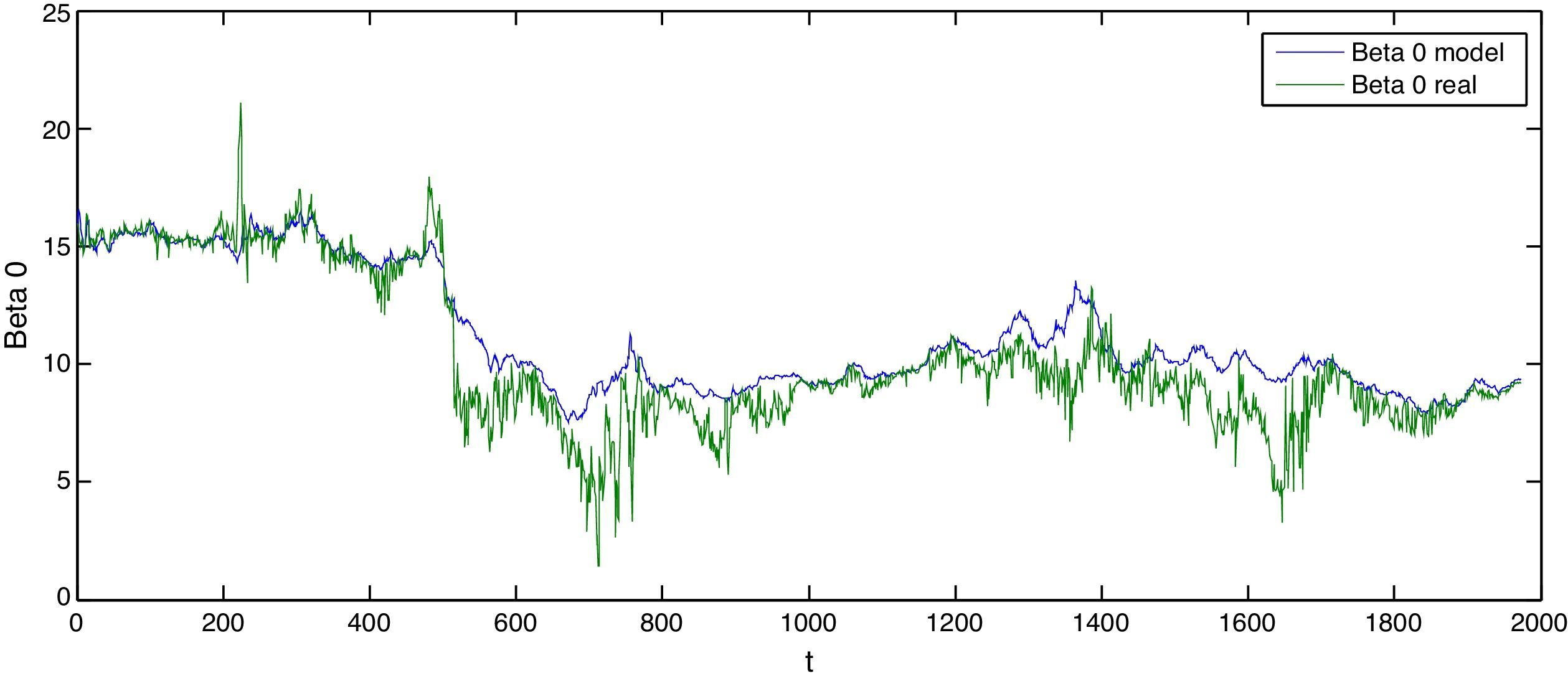
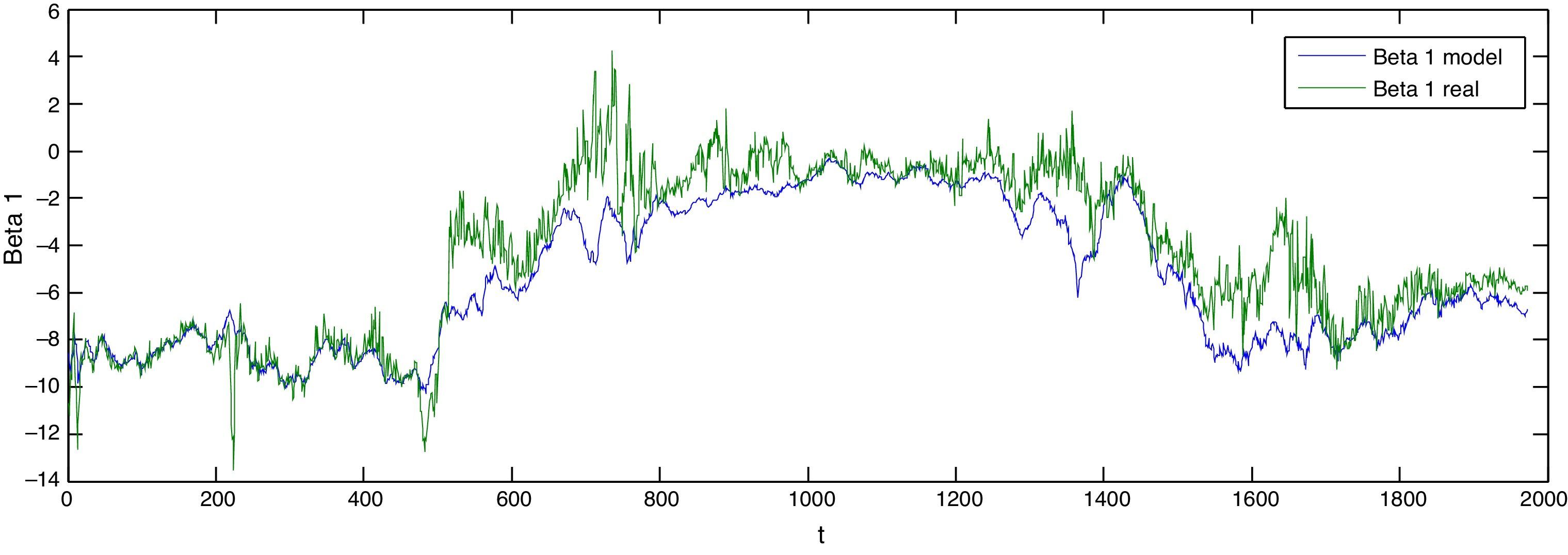
The green lines of Figures 2 and 3 show the real observations of the parameters β_0t and β_1t whereas the blue line shows the result of the estimation process. It is important to highlight that the model shows the tendency that real observations follow. Even though the existence of an estimation error of those parameters is evidenced, the yields results that form the term structure adjust importantly thanks to the process resourcefulness.

Figure 2.

Estimated beta 0 vs. real beta 0

Figure 2 shows the comparison of the estimated beta zero vs. the real parameters being the green line the real parameter and the blue line the estimated. Authors estimations based on the model proposed (blue line) and Nelson and Siegel's parameter for Colombia provided by INFOVAL (green line).

Figure 3.

Estimated beta 1 vs. real beta 1

Figure 3 shows the comparison of the estimated beta 1 vs. the real parameters being the green line the real parameter and the blue line the estimated.

Authors estimations based on the model proposed (blue line) and Nelson and Siegel's parameter for Colombia provided by INFOVAL (green line).

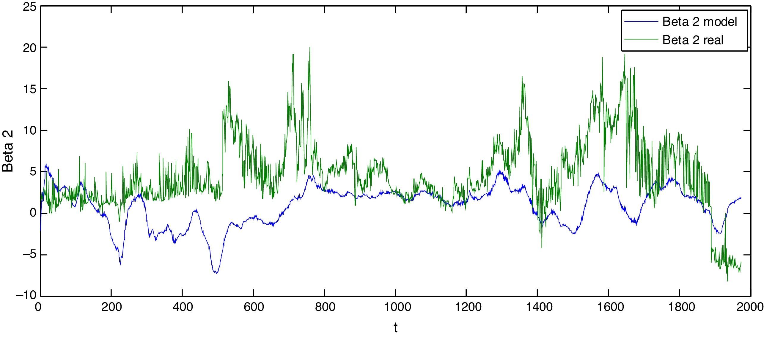
The blue line of Figure 4 shows the results of the parameter estimation β_2t which differs from the real observations shown in the green line, this is due to the higher weight of the lambda factor in the loading of this parameter. However, it is important to highlight the adjustment to the tendency.

Figure 4.

Estimated beta 2 vs. real beta 2

Figure 4 shows the comparison of the estimated beta 2 vs. the real parameters being the green line the real parameter and the blue line the estimated.

Authors estimations based on the model proposed (blue line) and Nelson and Siegel's parameter for Colombia provided by INFOVAL (green line).

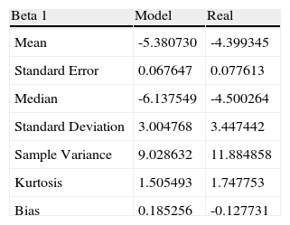
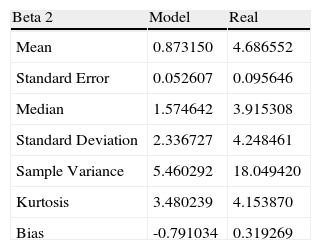
The divergences in the parameter estimations compared to the real observations are due to the effect that lambda has on each loading, this could be seen in Tables 1–3.

Table 1.

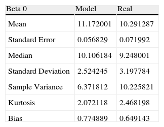
Statistics of estimated parameter β_0t vs. real.

Beta 0	Model	Real
Mean	11.172001	10.291287
Standard Error	0.056829	0.071992
Median	10.106184	9.248001
Standard Deviation	2.524245	3.197784
Sample Variance	6.371812	10.225821
Kurtosis	2.072118	2.468198
Bias	0.774889	0.649143

Table 1 shows the statistics of the estimated parameter beta zero vs. the real parameter.

Authors calculations.

Table 2.

Statistics of estimated parameter β_1t vs real.

Beta 1	Model	Real
Mean	-5.380730	-4.399345
Standard Error	0.067647	0.077613
Median	-6.137549	-4.500264
Standard Deviation	3.004768	3.447442
Sample Variance	9.028632	11.884858
Kurtosis	1.505493	1.747753
Bias	0.185256	-0.127731

Table 2 shows the statistics of the estimated parameter beta 1 vs. the real parameter.

Authors calculations.

Table 3.

Statistics of estimated parameter β_2t vs. real.

Beta 2	Model	Real
Mean	0.873150	4.686552
Standard Error	0.052607	0.095646
Median	1.574642	3.915308
Standard Deviation	2.336727	4.248461
Sample Variance	5.460292	18.049420
Kurtosis	3.480239	4.153870
Bias	-0.791034	0.319269

Table 3 shows the statistics of the estimated parameter beta 2 vs. the real parameter.

Authors calculations.

After obtaining the parameters, these and the loadings are in charge of determining the form of the term structure of the interest rates, we proceeded to calculate the zero-coupon yield curve for the Colombian economy given the expiration times determined from the beginning, and continue the process comparing them to the real expiration times. The next figures show the yields in three representative points: the short, medium and long part of the curve.

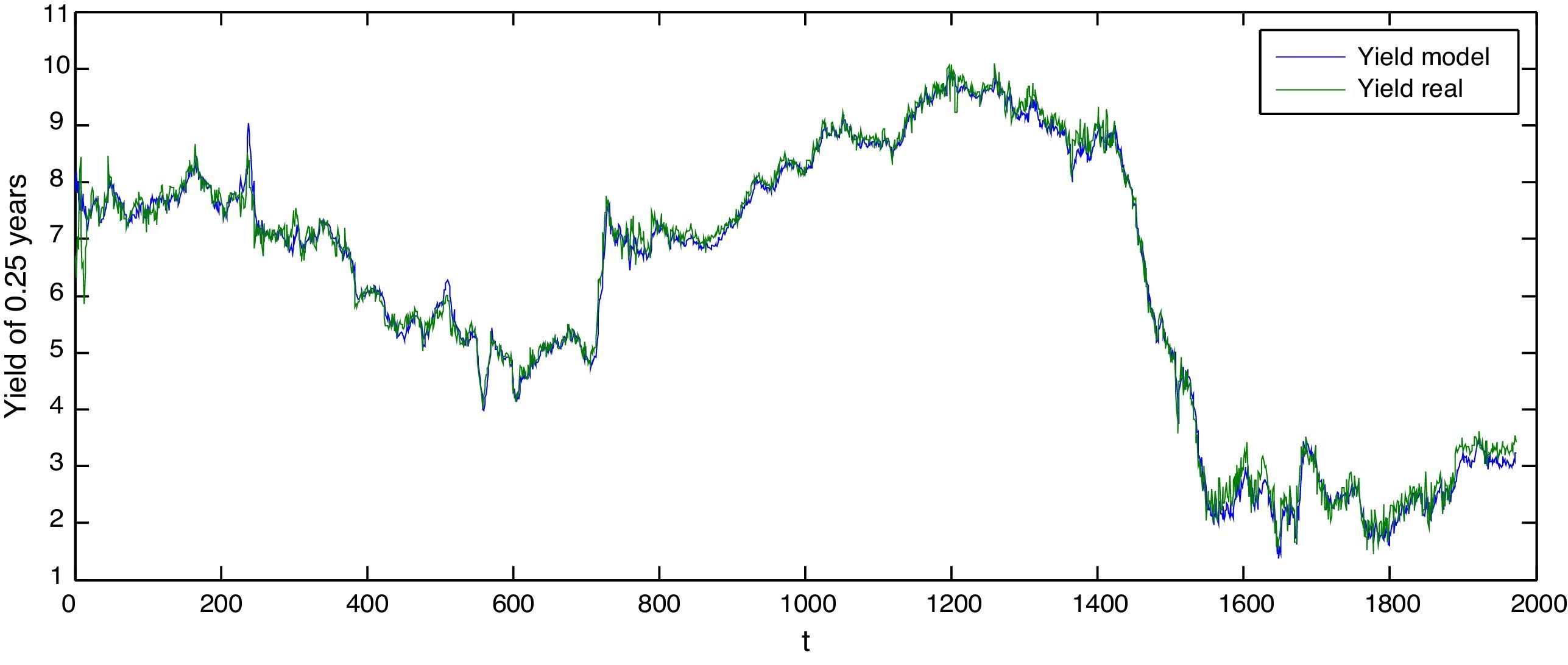
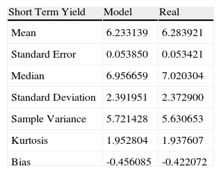
Figure 5 shows the behavior of the yield estimation of the curve's short part in green contrasted with the real data in blue. Thus, the forecasting adjustment is evidenced in Table 4, which presents the statistics of the obtained results.

Figure 5.

Estimated yield vs real with expiration in 0.25 years

Figure 5 shows the estimated and real yields in the short part of the curve being the green line the real yield and the blue one the estimated.

Authors estimations based on the model proposed (blue line) and Nelson and Siegel's parameter for Colombia provided by INFOVAL (green line).

Table 4.

Estimated yield statistics vs. real with expiration in 0.25 years.

Short Term Yield	Model	Real
Mean	6.233139	6.283921
Standard Error	0.053850	0.053421
Median	6.956659	7.020304
Standard Deviation	2.391951	2.372900
Sample Variance	5.721428	5.630653
Kurtosis	1.952804	1.937607
Bias	-0.456085	-0.422072

Table 4 shows the statistics of the estimated short term yield vs. the real yield.

Authors calculations.

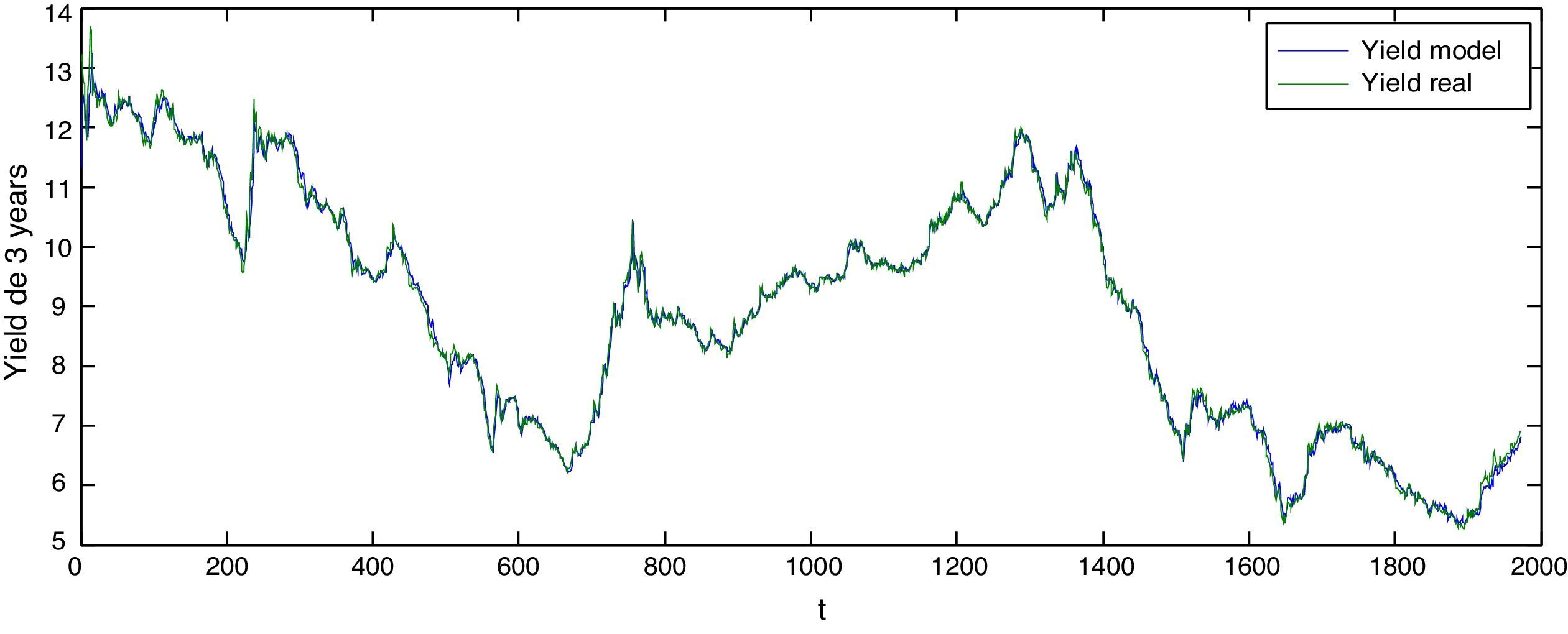
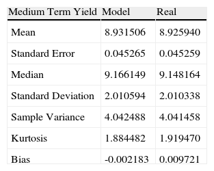
Figure 6 shows the behavior of the yield estimation of the midpart of the curve in green contrasted with the real data in blue. Note the statistics of Table 5 that present the forecasting adjustment.

Figure 6.

Estimated yield vs. real yield with expiration in 3 years

Figure 6 shows the estimated and real yields in the medium part of the curve being the green line the real yield and the blue one the estimated.

Authors estimations based on the model proposed (blue line) and Nelson and Siegel's parameter for Colombia provided by INFOVAL (green line).

Table 5.

Estimated yield statistics vs. real with expiration in 3 years.

Medium Term Yield	Model	Real
Mean	8.931506	8.925940
Standard Error	0.045265	0.045259
Median	9.166149	9.148164
Standard Deviation	2.010594	2.010338
Sample Variance	4.042488	4.041458
Kurtosis	1.884482	1.919470
Bias	-0.002183	0.009721

Table 5 shows the statistics of the estimated short term yield vs. the real yield.

Authors calculations.

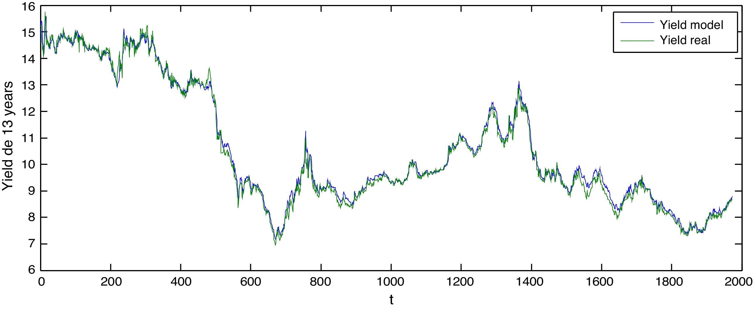
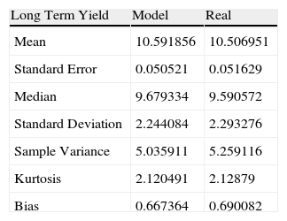
Figure 7 and Table 6 show the behavior of the yields estimation in the long part of the curve in green compared with the real data in blue. Table 7

Figure 7.

Estimated yield vs. real with expiration in 13 years

Figure 7 shows the estimated and real yields in the long part of the curve being the green line the real yield and the blue one the estimated.

Authors estimations based on the model proposed (blue line) and Nelson and Siegel's parameter for Colombia provided by INFOVAL (green line).

Table 6.

Estimated yield statistics vs. real with expiration in 13 years.

Long Term Yield	Model	Real
Mean	10.591856	10.506951
Standard Error	0.050521	0.051629
Median	9.679334	9.590572
Standard Deviation	2.244084	2.293276
Sample Variance	5.035911	5.259116
Kurtosis	2.120491	2.12879
Bias	0.667364	0.690082

Table 6 shows the statistics of the estimated long term yield vs. the real yield.

Authors calculations.

Table 7.

Results of the adjustment proofs of the yields.

Term	MAPE	RMSE
Short Term Yield	0.004843	0.576248
Medium Term Yield	-0.000524	0.215949
Long Term Yield	-0.0048875	0.574961

Table 7 shows the adjustment tests for the estimated yields obtained with the model.

Authors calculations.

Observations indicate that the behavior of the yields estimations in the model is more adjusted that in the parameter estimations compared to their observed pairs, this is due to the resourcefulness and efficiency that the Kalman filter provides to the model.

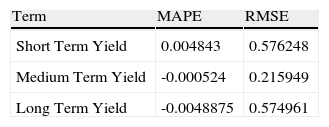
In addition to this, adjustment proofs of the yields were done for each of the analyzed expiration periods, which evidenced good behavior in the forecasting as it is shown in the following table.

4

Conclusions

This paper presented how to obtain a zero-coupon yield curve forecasting for Colombia, which is framed by law in the Nelson and Siegel model (1987) through the use of two resources. The first is the use of the Diebold and Li model established in 2006, which proposes a reparametrization of the Nelson and Siegel model (1987) in three latent factors, level, slope and curvature. And the second, and most important, a mathematical tool that is formed by a set of recursive equations that can be obtained by a forecasting and an error correction.

Given the resourcefulness and efficiency in the error correction that provides the Kalman filter, it was possible to obtain a well-adjusted dynamic forecasting for a horizon t +1, as it is evidenced in the tables that complement the figures throughout this paper.

Regarding the theoretical framework, Diebold and Li (2006) proposed, the estimation of a representative lambda for the studied economy in order to facilitate modeling, our research required to obtain. However, it was observed how the forecasting of the term structure parameters is affected as the loadings contain a great contribution to lambda. Nevertheless, the methodology to calculate the zero-coupon yields curve estimated from the forecasting of parameters are extremely close to the real observations, due to the self-correction property of the model.

After analyzing the results shown graphically and in the tables, we consider that the achieved forecasting by the model described in this paper is accurate for a period ahead, especially if the forecasting can capture the tendency followed by the observations that were compared with the obtained results.

Finally, additional analysis can be inferred from this research, such as the forecasting evaluation with forecasts in longer periods of time in order to evaluate if the efficiency is as accurate as the results obtained in this document.