A sustained high growth rate of gross domestic product at a low inflation is one of the main goals of the majority of macroeconomic policies, so keeping the price stability plays an important role in determining the growth rate of output. This paper empirically investigates effects of fiscal deficit and broad money M2 supply on inflation in Asian countries, namely Bangladesh, Cambodia, Indonesia, Malaysia, Pakistan, Philippines, Sri Lanka, Thailand, and Vietnam in the period of 1985-2012. By applying the Pooled Mean Group (PMG) estimation-based error correction model and the panel differenced GMM (General Method of Moment) Arellano-Bond estimator, the study finds out broad money M2 supply has significantly positive impact on inflation only in the method of PMG estimation whereas fiscal deficit, government expenditure and interest rate are the statistically significant determinants of inflation in both methods of estimation
El sostenimiento de una elevada tasa de crecimiento del producto bruto interno a baja inflación es uno de los principales objetivos de la mayoría de las políticas macroeconómicas, por lo que el mantenimiento de la estabilidad de los precios juega un papel relevante en la determinación del índice de crecimiento del output. Este documento investiga empíricamente los efectos del déficit fiscal y el suministro amplio de dinero M2 sobre la inflación en los países asiáticos, en concreto Bangladesh, Camboya, Indonesia, Malasia, Paquistán, Filipinas, Sri Lanka, Tailandia, y Vietnam durante el periodo comprendido entre 1985 y 2012. Aplicando el modelo de corrección basado en la estimación de Pooled Mean Group (PMG) y el estimador Arellano-Bond del Método Generalizado de Momentos (MGM) del panel diferenciado, el estudio llega a la conclusión de que el amplio suministro de dinero M2 tiene un impacto considerablemente positivo sobre la inflación utilizando únicamente el método de la estimación de PMG, mientras que el déficit fiscal, el gasto gubernamental y los tipos de interés constituyen determinantes estadísticamente significativos de la inflación en ambos métodos de cálculo.
A major objective of macroeconomic policies is to foster economic growth and to keep inflation on a low level. The stability of price is one of the factors in determining the growth rate of an economy; hence, the monetary authorities of many countries implement monetary policies to maintain inflation at a desirable rate. A very high inflation affects the economy drastically, but there is some evidence that moderate inflation also slows down growth (Temple, 2000). However, the high level of inflation stems from not only instruments of monetary policy (money supply, interest rate, etc.) but also the effects of fiscal policy (fiscal deficit, government expenditure, etc.). Indeed, Fischer, Sahay, & Végh (2002) showed that fiscal deficit is one of main drivers of high inflation.
Most of selected Asian countries have high relatively levels of fiscal deficit and money supply as governments increase spending to foster economic growth and create employment. According to Asian Development Bank (2013), the average shares of budget deficit and broad money M2 supply to GDP in 2012 in these countries is -3.9% and 71.6% respectively in which the highest ratios of fiscal deficit belong to Pakistan (-6.64%), Sri Lanka (-6.4%) and Bangladesh (-4.56%) while that of broad money M2 supply occur at Malaysia (142%), Thailand (124.8%) and Vietnam (108.4%). By new econometric techniques, the study will define significant determinants of inflation in order to suggest some recommendations about macroeconomic policies related to inflation.
The purpose of this paper is to apply the PMG-based error correction model and the panel differenced GMM Arellano-Bond estimation to investigate effects of fiscal deficit and broad money M2 supply on inflation in Asian countries, namely Bangladesh, Cambodia, Indonesia, Malaysia, Pakistan, Philippines, Sri Lanka, Thailand, and Vietnam in the period of 1985–2012.
The remainder of this paper will be proceed as follows: Section 2 outlines a review of literature about effects of fiscal deficit and money supply on inflation; Section 3 describes the methodology and data; Section 4 presents results and discussion, and the final section is the conclusion and policy implications.
2Literature review2.1The effect of fiscal deficit on inflationSeveral studies have exploited both the time and cross-sectional dimensions of data (panel data) to examine the relationship between fiscal deficits and inflation. Karras (1994) investigates the effects of budget deficits on money growth, inflation, investment and real output growth using annual data from a sample of 32 countries in the period of 1950-1989 and finds that deficits are not inflationary. However, Cottarelli et al. (1998) find a significant impact of fiscal deficits on inflation in industrial and transition economies by using the dynamic panel data model in 47 countries from 1993 to 1996.
Fischer et al. (2002), using the data set of 94 developing and developed countries from 1960 to 1995, find that the relationship between fiscal deficits and inflation is only strong in high-inflation countries during high-inflation episodes, and weak in low-inflation countries and in high-inflation countries during low-inflation episodes.
Catão and Terrones (2005) apply the pooled mean group estimation method to a data set spanning 107 countries over the 1960-2001 period. It is shown that, empirically, deficits have an impact on inflation and such an impact is stronger in high-inflation or developing countries. As mentioned by Catão and Terrones (2005), developing countries with less efficient tax collection, political instability, and limited access to external borrowing tend to have a lower relative cost of seigniorage and thus a higher inflation tax.
Lin and Chu (2013) applies the dynamic panel quartile regression (DPQR) model under the autoregressive distributional lag (ARDL) specification, and examines the deficit-inflation relationship in 91 countries from 1960 to 2006. The DPQR model estimates the impact of deficits on inflation at various inflation levels and allows for a dynamic adjustment with the ARDL specification. The empirical results note that the fiscal deficit has a strong impact on inflation in high-inflation episodes, and has a weak impact in low-inflation episodes.
Jayaraman and Chen (2013) investigates the relationship between budget deficits and inflation in the four Pacific Island countries (PICs) by undertaking an empirical study of relationship between budget deficits in the four PICs through a panel econometric analysis. A multivariate framework is adopted with a view to avoiding bias arising out of omission of relevant variables and the methodology employed for estimating a long-run relationship between budget deficits and inflation is the Westerlund error correction based panel co-integration test procedure. The study's findings confirm the existence of a strong, direct relationship between budget deficits and inflation in all four PICs.
2.2Effect of money supply on inflationMost of empirical studies confirm a strong impact of money supply on inflation. McCandless & Weber (1995) examine data for 110 countries over a 30-year period. The study shows that there is a high (almost unity) correlation between the rate of growth of the money supply and the rate of inflation in long term. With regard to the relationship between money and prices, King (2002) shows that the strong correlation between them disappears as the time horizon shortens indicating that the effects of money growth should emerge in the changes in real variables. According to Walsh (2003), the high correlation between inflation and the growth rate of money supply supports the quantity-theoretic argument that the growth of money supply leads to an equal rise in the price level.
Nassar (2005) uses a two-sector model to estimate the relationship between prices, money, and the exchange rate for quarterly data in Madagascar in the period of 1982-2004. The results show that the money supply has significantly positive impact on inflation.
Oomes and Ohnsorge (2005) investigates the impact of money demand on inflation for monthly data in Russia from April 1996 to January 2004 by using the error correction model. The results confirm that an excess supply of effective broad money is inflationary while other excess money measures are not and that effective broad money growth has the strongest and most persistent effect on short-run inflation.
Pelipas (2006) empirically investigates the money demand and inflation Belarus on the basis of the quarterly data for 1992-2003. Using co-integrated VAR and equilibrium correction model, the study notes the money supply is significantly positive correlated with inflation.
Hossain (2010) investigates the behavior of broad money demand in Bangladesh using annual data over the period of 1973-2008 by using the Johansen co-integration test and the error correction model. Empirical results suggest the existence of a causal relationship between money supply growth and inflation.
3Methodology and data3.1MethodologyPesaran et al. (1997; 1999) proposed the PMG estimator that allows the short-term parameters to be heterogeneous between groups while imposing homogeneity of the long-term coefficients between countries. It is one advantage of PMG estimator. Furthermore, the PMG estimator highlights the adjustment dynamic between the short-run and the long-run. The heterogeneity of short-run slope coefficients allows the dynamic specification to differ across countries. However, the drawback of PMG estimator is that it cannot deal with the endogeneity of variables in the model.
The PMG estimation-based error correction model requires an existence of co-integration between dependent variable and explanatory variables. So, the study first tests the stationary of the variables by using the Fisher tests, developed by Maddala and Wu (1999) and then applies the co-integration test of Westerlund (2007).
The dynamic panel GMM estimation uses the appropriate lags of the instrumented variables to generate internal instruments and employs the pooled dimension of the panel data. So it does not put restrictions on the length of each individual time dimension in the panel. This enables use of suitable lag structure to exploit the dynamic specification of the data. However, this approach still has some important shortcomings (Anshasy, 2012). First, it only allows the intercepts —not slopes— to vary across groups. Pesaran et al. (1997; 1999) argued that the assumption of homogeneity of slope parameters may not be proper when the time dimension of the panel is short. Second, cross-sectional dependence is not addressed.
3.2The PMG estimation-based error correction modelWhere Y is inflation; Sit-1 is the deviation from long-run equilibrium at any period for group i, and ϕ is the error-correction (speed of adjustment) coefficient. The vector θ captures the long-run coefficients which do not vary across groups; these coefficients represent the long-run elasticity of inflation with respect to each variable in Xit-1. The short-run responses of the X variables are captured by the vector δ. ηi is an unobserved time-invariant, country-specific effect and ζit is an observation-specific error term.
3.3The panel differenced GMM Arellano-Bond estimationWhere Y is inflation in first difference; X is a vector of variables in first difference including variables of fiscal policy (fiscal deficit and government expenditure), variables of monetary policy (broad money M2 supply and interest rate) and some control variables (real GDP per capita, exchange rate and trade openness); ηi is an unobserved time-invariant, country-specific effect and ζit is an observation-specific error term.
The dynamic characteristics in (2) show that the country-specific fixed effects can be correlated with the lagged dependent variable and some explanatory variables may be endogenous. It can make OLS inconsistency and estimates bias. However the panel differenced Generalized Method of Moments (GMM) estimator, developed by Arellano and Bover (1995), and Blundell and Bond (1998), tackles these problems. It utilizes the lagged differences of the predetermined variable as instruments for their levels and the differences of the strictly exogenous variables (as in the standard IV procedure).
In addition, based on the information criterions BIC and AIC, the study uses lag orders K=2 identical for all cross-units, respecting the condition T>5+2K, which is important to guarantee the validity of the proposed tests, even with shot T samples (see Hurlin, 2004).
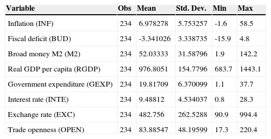
3.4DataThe data are extracted from annual data of Asian Development Bank (Key Indicators for Asia and the Pacific) for nine Asian countries, namely Bangladesh, Cambodia, Indonesia, Malaysia, Pakistan, Philippines, Sri Lanka, Thailand and Vietnam in the period of 1985-2012. The primary data include inflations; fiscal deficits (share of GDP), broad money M2 supply (share of GDP), real GDP per capita, government expenditure (share of GDP), interest rates, exchange rate (ratio of domestic currency and USD), exports (share of GDP) and imports (share of GDP). From the primary data, the study transfers into the secondary data including variables INF (inflations, percentage), BUD (fiscal deficits, percentage), M2 (broad money supply, percentage), RGDP (real GDP per capita, in natural logarithm form), GEXP (government expenditure, percentage), INTE (interest rates, percentage), EXC (exchange rates, in natural logarithm form) and OPEN (trade openness, percentage) in which RGDP and EXC are defined in form of natural logarithm multiplied with 100 and OPEN is the sum of shares of exports and imports to GDP. The descriptive statistics of all variables is described in the Table 1.
Descriptive statistics.
| Variable | Obs | Mean | Std. Dev. | Min | Max |
|---|---|---|---|---|---|
| Inflation (INF) | 234 | 6.978278 | 5.753257 | -1.6 | 58.5 |
| Fiscal deficit (BUD) | 234 | -3.341026 | 3.338735 | -15.9 | 4.8 |
| Broad money M2 (M2) | 234 | 52.03333 | 31.58796 | 1.9 | 142.2 |
| Real GDP per capita (RGDP) | 234 | 976.8051 | 154.7796 | 683.7 | 1443.1 |
| Government expenditure (GEXP) | 234 | 19.81709 | 6.370099 | 1.1 | 37.7 |
| Interest rate (INTE) | 234 | 9.48812 | 4.534037 | 0.8 | 28.3 |
| Exchange rate (EXC) | 234 | 482.756 | 262.5288 | 90.9 | 994.4 |
| Trade openness (OPEN) | 234 | 83.88547 | 48.19599 | 17.3 | 220.4 |
Author elaboration (software output).
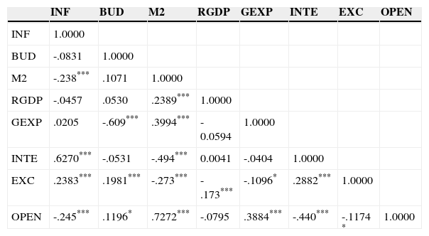
The matrix of Pearson correlation coefficients is summarized in Table 2. The results show that the pair of broad money M2 supply and trade openness has the biggest coefficient (0.7272). According to Evans (1996), the correlation level between them is relatively strong while that of others are moderate and weak. However, for the time series in finance, the correlation coefficient, lower than 0.8 is acceptable. Therefore, the study decides to use these all variables in the model.
The matrix of Pearson correlation coefficients.
| INF | BUD | M2 | RGDP | GEXP | INTE | EXC | OPEN | |
|---|---|---|---|---|---|---|---|---|
| INF | 1.0000 | |||||||
| BUD | -.0831 | 1.0000 | ||||||
| M2 | -.238*** | .1071 | 1.0000 | |||||
| RGDP | -.0457 | .0530 | .2389*** | 1.0000 | ||||
| GEXP | .0205 | -.609*** | .3994*** | -0.0594 | 1.0000 | |||
| INTE | .6270*** | -.0531 | -.494*** | 0.0041 | -.0404 | 1.0000 | ||
| EXC | .2383*** | .1981*** | -.273*** | -.173*** | -.1096* | .2882*** | 1.0000 | |
| OPEN | -.245*** | .1196* | .7272*** | -.0795 | .3884*** | -.440*** | -.1174 * | 1.0000 |
***, **, *: statistically significant at 1%, 5% and 10% respectively
Author elaboration (software output).
As mentioned in the Section 3 of Methodology and data, this paper applies the PMG estimation–based error correction model to analyse the effects of fiscal deficit and broad money M2 supply on inflation. Before carrying out it, the stationary tests and co-integration tests need to be done to make sure that all variables in the model are co-integrated.
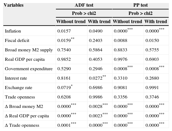
The results of stationary tests in Table 3 show that variables inflation, fiscal deficit, government expenditure, interest rate and exchange rate are significantly stationary at levels less than 10% while variables broad money M2 supply, real GDP per capita and trade openness are not stationary. It means that in this model some variables have integration of zero order I(0) and the others integration of first order I(1). Therefore, the study follows the Westerlund co-integration tests for dependent variable (inflation) and explanatory variables (the remaining variables).
Fisher type unit root tests with lags=2.
| Variables | ADF test | PP test | ||
|---|---|---|---|---|
| Prob>chi2 | Prob>chi2 | |||
| Without trend | With trend | Without trend | With trend | |
| Inflation | 0.0157 | 0.0490 | 0.0000*** | 0.0000*** |
| Fiscal deficit | 0.0159** | 0.2403 | 0.0088 | 0.0150 |
| Broad money M2 supply | 0.7540 | 0.5864 | 0.8833 | 0.5755 |
| Real GDP per capita | 0.9852 | 0.4053 | 0.9976 | 0.6903 |
| Government expenditure | 0.5290 | 0.2946 | 0.0008*** | 0.0008*** |
| Interest rate | 0.8161 | 0.0272** | 0.3310 | 0.2680 |
| Exchange rate | 0.0719* | 0.6986 | 0.9081 | 0.9991 |
| Trade openness | 0.6208 | 0.9986 | 0.3356 | 0.3746 |
| Δ Broad money M2 | 0.0000*** | 0.0028*** | 0.0000*** | 0.0000*** |
| Δ Real GDP per capita | 0.0000*** | 0.0023*** | 0.0000*** | 0.0000*** |
| Δ Trade openness | 0.0001*** | 0.0000*** | 0.0000*** | 0.0000*** |
***, **, *: statistically significant at 1%, 5% and 10% respectively.
Author elaboration (software output).
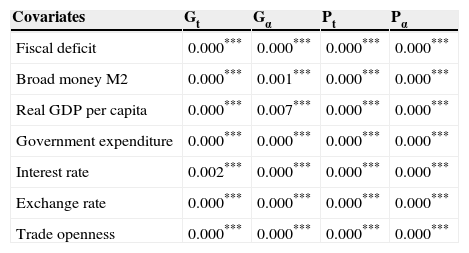
Table 4 presents Westerlund panel co-integration tests. When all four tests reject the null of no co-integration, a covariate is considered co-integrated with the dependent variable. So the results show that fiscal deficit, broad money M2 supply, real GDP per capita, government expenditure, interest rate, exchange rate and trade openness are co-integrated with inflation.
Westerlund panel co-integration tests. Normalized variable: Inflation.
| Covariates | Gt | Gα | Pt | Pα |
|---|---|---|---|---|
| Fiscal deficit | 0.000*** | 0.000*** | 0.000*** | 0.000*** |
| Broad money M2 | 0.000*** | 0.001*** | 0.000*** | 0.000*** |
| Real GDP per capita | 0.000*** | 0.007*** | 0.000*** | 0.000*** |
| Government expenditure | 0.000*** | 0.000*** | 0.000*** | 0.000*** |
| Interest rate | 0.002*** | 0.000*** | 0.000*** | 0.000*** |
| Exchange rate | 0.000*** | 0.000*** | 0.000*** | 0.000*** |
| Trade openness | 0.000*** | 0.000*** | 0.000*** | 0.000*** |
***, **, *: statistically significant at 1%, 5% and 10% respectively.
Author elaboration (software output).
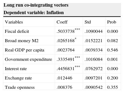
The estimation of PMG-based error correction model is expressed in Table 5. In long run, the effects of fiscal deficit, government expenditure and interest rate on inflation are significantly positive at level of 1% while that of broad money M2 supply only at level of 10%. Impacts of fiscal deficit and broad money M2 supply on inflation are consistent with previous empirical studies. In fact, Fischer et al. (2002), Catão and Terrones (2005), Lin and Chu (2013) and Jayaraman and Chen (2013) found fiscal deficit has strongly positive influence on inflation and Nassar (2005), Oomes and Ohnsorge (2005), Pelipas (2006) and Hossain (2010) confirmed broad money supply are positively correlated with inflation.
Error Correction Model (PMG estimations, 1985 - 2012).
| Long run co-integrating vectors | |||
|---|---|---|---|
| Dependent variable: Inflation | |||
| Variables | Coeff | Std | Prob |
| Fiscal deficit | .5033738*** | .1090044 | 0.000 |
| Broad money M2 | .0265168* | .0152221 | 0.082 |
| Real GDP per capita | .0023764 | .0039334 | 0.546 |
| Government expenditure | .3335491*** | .1016084 | 0.001 |
| Interest rate | .4456831*** | .0762972 | 0.000 |
| Exchange rate | .012446 | .0097201 | 0.200 |
| Trade openness | .008376 | .0090542 | 0.355 |
| Short run dynamics (mean countries) | |||
|---|---|---|---|
| Dependent variable: Inflation growth | |||
| Error correction | -.8017676*** | .0786158 | 0.000 |
| Δ Fiscal deficit | -.2210842 | .1765845 | 0.211 |
| Δ Broad money M2 | -.3611816*** | .1107341 | 0.001 |
| Δ Real GDP per capita | -.1666343 | .1119978 | 0.137 |
| Δ Government expenditure | -.4283285* | .2559721 | 0.094 |
| Δ Interest rate | .4868342** | .2441704 | 0.046 |
| Δ Exchange rate | -.0152209 | .0501708 | 0.762 |
| Δ Trade openness | .0240599 | .0380454 | 0.527 |
| Cons | -9.47206*** | 1.810749 | 0.000 |
| Obs | 225 | ||
| Log likelihood | -478.5965 | ||
***, **, *: statistically significant at levels of 1%, 5% and 10% respectively.
Author (software output).
According to Bajo-Rubio, Díaz-Roldán, & Esteve (2009), the Fiscal Theory of the Price Level (FTPL) takes into account monetary and fiscal policy interactions and assumes that fiscal policy may determine the price level, even if monetary authorities pursue an inflation targeting strategy. This approach allows fiscal policy to set primary surpluses/deficits to follow an arbitrary process, not necessarily compatible with solvency. Therefore, the budget surplus/deficit path would be exogenous, and the endogenous adjustment of the price level would be required in order to achieve fiscal solvency. In this context, fiscal policy becomes “active”, with budget surpluses turning to be the nominal anchor; whereas monetary policy becomes “passive” and can only control the timing of inflation. Therefore, an increase in fiscal deficits as well as in government expenditure, two important instruments of fiscal policy, lead to high inflation.
However, the influence of interest rate on inflation can be explained in two ways. One is based on cost of capital. According to Asgharpur, Kohnehshahri, & Karami (2007), the increased interest rate raises the cost of capital that results in higher production costs. This changes raise inflation by shifting the aggregate supply curve to the left side. The second, the changing interest rate impacts on inflation through influencing the money volume. In the endogenous money models which money supply is a function of interest rate, the money supply is increased when interest rate goes up. So, according to quantity theory of money, the more money supply results in inflation in the short and long run.
In short run, broad money M2 supply, government expenditure and interest rate are significant determinants of inflation. In addition, the error correction coefficient is significantly negative at level of 1%, confirming that there exists a co-integration long run relationship in at least one of the panel countries. Accordingly, the speed of adjustment in the short run to reach equilibrium level in the long run is 80.17%/year.
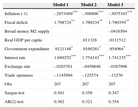
To confirm whether the above results of PMG estimator is reliable or not, the study continues to follow the differenced panel GMM Arellano-Bond estimations. The estimated results are outlined in Table 6.
Differenced panel GMM Arellano-Bond estimations. Dependent variable: Inflation.
| Model 1 | Model 2 | Model 3 | |
|---|---|---|---|
| Inflation (-1) | -.2973489*** | -.308896*** | -.3075103*** |
| Fiscal deficit | 1.798724** | 1.769234** | 1.790359** |
| Broad money M2 supply | -.0416564 | ||
| Real GDP per capita | .011328 | .0111512 | |
| Government expenditure | .9121148* | .9160281* | .954064* |
| Interest rate | 1.689252*** | 1.754143*** | 1.741235*** |
| Exchange rate | -.0293761 | -.0456646 | -.0387998 |
| Trade openness | -.1145094 | -.125574 | -.13276 |
| Obs | 207 | 207 | 207 |
| Sargan test | 0.301 | 0.359 | 0.347 |
| AR(2) test | 0.362 | 0.321 | 0.354 |
***, **, *: statistically significant at levels of 1%, 5% and 10% respectively.
Author elaboration (software output).
To check the robustness of the panel differenced GMM Arellano-Bond estimation, the estimated results are usually verified by removing/adding some variables. Accordingly, this estimation begins at Model 1, then continues with Model 2 and ends at Model 3 (the full variables model). All results from Model 1, 2, 3 show that estimated coefficients are approximately unchanged. It confirmed that results of the panel GMM estimation are strongly robust. Except for impact of broad money M2, effects of fiscal deficit, government expenditure and interest rate on inflation are completely consistent with the estimated results of PMG estimator, implying the impact of broad money M2 on inflation is not significant in panel GMM estimation. Accordingly, increase in money supply does not necessarily cause inflation. With increase in money supply interest rate is likely to fall and decline in interest rate may lead to higher investment and output and in that case money supply is not inflationary.
5Conclusion and policy implicationsThe study applied two methods of estimation, the PMG estimation and the differenced panel GMM Arellano-Bond estimation, to analyze the effects of fiscal deficit and broad money M2 supply on inflation in Asian countries, namely Bangladesh, Cambodia, Indonesia, Malaysia, Pakistan, Philippines, Sri Lanka, Thailand, and Vietnam in the period of 1985-2012. The estimated results show that broad money M2 supply has significantly positive impact on inflation only in the method of PMG estimation whereas fiscal deficit, government expenditure and interest rate are the statistically significant determinants of inflation in both methods of estimation.
The policy implications of empirical results are very clear. Broad money M2 supply, fiscal deficit, government expenditure and interest rate are positively correlated with inflation. Therefore, when applying the fiscal and monetary policies to foster the economy, governments of Asian countries should be careful at money supply, fiscal deficit, government expenditure and interest rate because they can contribute to high inflation for the economy.


