Measuring market liquidity in US fixed income markets: A new synthetic indicator

Abstract

We propose a new synthetic liquidity indicator that summarizes the information of a broad set of market liquidity measures for both sovereign and corporate fixed income markets in the US. Our index is based on seventeen liquidity measures that cover the main dimensions of market liquidity. The methodology to compute the index consists of two steps. First, we carry out a transformation of the individual liquidity measures based on that of Holló et al. (2012) for the CISS—Composite Indicator of Systemic Stress—and second, we weight the transformed variables using a principal component analysis. The indicator shows that liquidity in US fixed income markets has been impaired after the global financial crisis mainly as a result of weaker liquidity conditions in US Treasury markets, whereas those in the corporate debt market remained stable.

1

Introduction

The concept of liquidity is broad and complex. This has been acknowledged by many researchers in the field. For example, Shin (2005) states that liquidity defies a simple definition and Tirole (2011) explains why liquidity cannot easily be apprehended through a single statistic. Hence, in this paper we focus only on a particular type of liquidity—i.e. market liquidity—and we use a composite indicator that captures various dimensions of liquidity. Market liquidity may be defined as the easiness with which market participants can buy or sell an asset in a market without affecting its price (Elliot, 2015). The definition of market liquidity differs from that of monetary liquidity, related to central banks’ monetary aggregates, or from funding liquidity, which is the ability to obtain funding for a position in a risky asset (Brunnermeier and Pedersen, 2009).

In recent years, episodes of financial market strains and heightened volatility have been increasingly associated with discussions of the degree of liquidity in specific market segments. This was the case with the so-called “taper tantrum” in the second quarter of 2013 and the October 2014 “flash crash” in US Treasury markets.¹ Overall, market liquidity has been receiving a growing attention, given its apparent decline in some markets (IMF, 2015; Fender and Lewrick, 2015) and the possibility that impaired liquidity may have been one of the main drivers of these volatility spikes (Adrian et al., 2015).² Recently, a report published by the US Office of Financial Research (Office of Financial Research, 2015) showed that liquidity has been declining in a number of US markets in recent years, including the most liquid ones. The report suggested that this decline may amplify shocks in financial markets and impair financial stability. Its assessment was rather timely: Actual market developments around the report's publication in mid-December 2015—when turmoil hit US high-yield bond markets and three investment funds suspended redemptions—were linked to liquidity strains in certain segments of US corporate bond markets.

Measuring market liquidity is not an easy task, as its definition embodies several dimensions. In particular, Sarr and Lybek (2002) summarize the five characteristics that characterize market liquidity, namely tightness, immediacy, depth, breadth and resilience. The concept of tightness refers to transaction costs, which are supposed to be low in liquid markets, whereas immediacy characterizes those markets where trades are executed quickly and in an orderly manner. Depth is linked to the number of orders, while breadth allows orders to flow with a minimal impact in prices, even if they are large. Finally, in a resilient market, prices are able to move rapidly to new equilibrium levels; hence, resilience is closely related to market efficiency (Bernstein, 1987).

Given the heterogeneity of the characteristics behind the definition of market liquidity, there is a large number of indicators that have been proposed to monitor its various aspects. Some of them relate to plain transaction costs (“bid-ask” spreads), while others comprise more sophisticated measures that consider volume and price sensitivities of financial assets.³ The result is a plethora of indicators that usually gives different signals and does not allow for an unequivocal assessment of how liquidity conditions are evolving.

In addition, none of these single indicators can simultaneously capture all dimensions of market liquidity (Amihud and Mendelson, 1991). In this paper, we propose a synthetic liquidity index to overcome this problem. Although the literature of composite indicators has been traditionally devoted to evaluate financial stress—see Kliesen et al. (2012) for a recent survey on these indicators—, we use this framework to construct a liquidity index based on individual liquidity indicators. Previous literature on this type of liquidity indexes is scarce. As far as we know, only Adrian et al. (2015a) also calculate a liquidity composite indicator for US fixed income markets. Our proposed indicator is robust to the different scales of the individual indexes and encompasses all liquidity characteristics. Nevertheless, as liquidity is an unobservable variable, there is no reliable benchmark to assess liquidity conditions, which constitutes one of the main challenges to construct such an index.

Our index is based on liquidity indicators for two main fixed-income markets. Namely, the US Treasury market (i.e. the segment with maturities close to 10 years) and the US corporate bond market for both investment grade and high yield (IG and HY respectively onwards). Our choice for these markets is motivated by the fact that they have been at the centre of recent discussions in both academia and the financial industry on the significance of strains in market liquidity. Moreover, the outstanding amount of these debt securities (USD 20.8 trillion) represents a substantial share of the whole U.S fixed income markets (52% of total in the second quarter of 2015).⁴

The main contribution of this paper to the literature is twofold. First, to the best of our knowledge, it is the first empirical application that employs the methodology of particular financial stress indices to develop a liquidity index that encompasses both government and corporate debt securities. Second, the proposed index combines the main aspects related to market liquidity, so that the specific liquidity characteristic that drives liquidity conditions in both markets can be identified.

The remainder of the paper is structured as follows. First, Section 2 describes the selection of liquidity indicators which we use to construct the synthetic indicator and reports some initial findings. Section 3 covers the methodology underlying the composite liquidity index. Section 4 discloses the evolution of the proposed index during the last 10 years. Finally, Section 5 concludes.

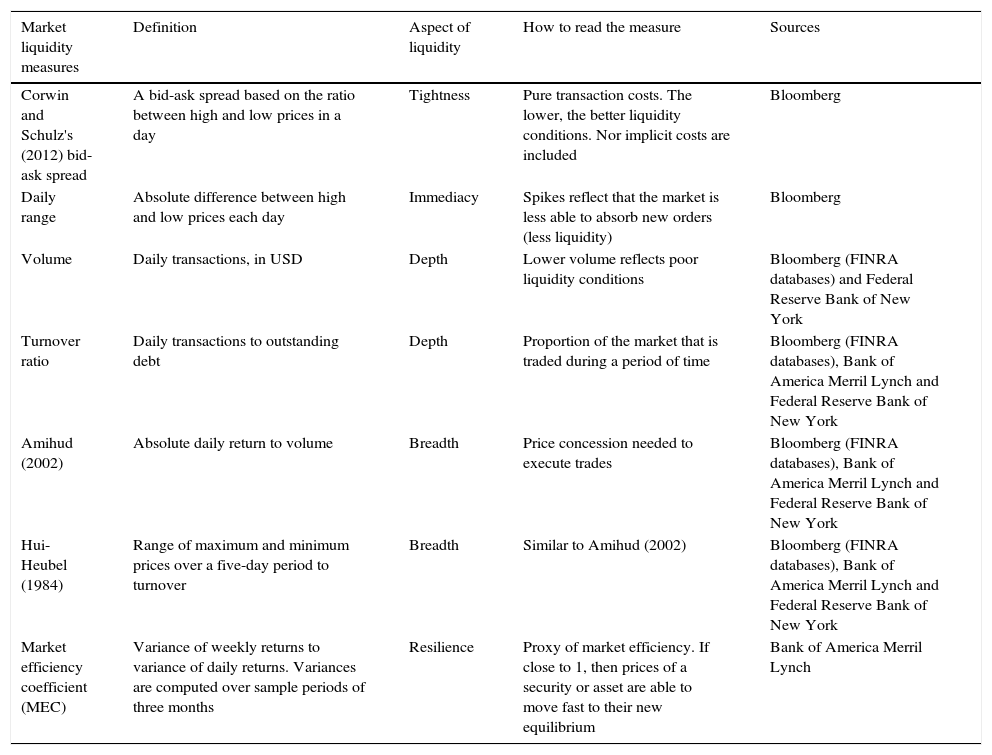
2

Market liquidity indicators

2.1

Selection of market liquidity indicators

Among the variety of liquidity metrics that are available, we have chosen seven to construct a synthetic index. We use these indicators for three markets, namely the US Treasury market and the US corporate IG and HY markets. All in all, we compute seventeen liquidity indicators in total for these markets, as some indicators are not available.⁵ Our selection allows capturing the five main characteristics of market liquidity, that is, tightness, immediacy, depth, breadth and resilience. Table 1 provides further details on the individual indicators and their respective data sources. We calculate the seventeen measures on a weekly basis. The sample period runs from July 20, 2005 to October 21, 2015, so that the sample size is T = 537.

Table 1.

Market liquidity measures used in the construction of the synthetic liquidity index.

Market liquidity measures	Definition	Aspect of liquidity	How to read the measure	Sources
Corwin and Schulz's (2012) bid-ask spread	A bid-ask spread based on the ratio between high and low prices in a day	Tightness	Pure transaction costs. The lower, the better liquidity conditions. Nor implicit costs are included	Bloomberg
Daily range	Absolute difference between high and low prices each day	Immediacy	Spikes reflect that the market is less able to absorb new orders (less liquidity)	Bloomberg
Volume	Daily transactions, in USD	Depth	Lower volume reflects poor liquidity conditions	Bloomberg (FINRA databases) and Federal Reserve Bank of New York
Turnover ratio	Daily transactions to outstanding debt	Depth	Proportion of the market that is traded during a period of time	Bloomberg (FINRA databases), Bank of America Merril Lynch and Federal Reserve Bank of New York
Amihud (2002)	Absolute daily return to volume	Breadth	Price concession needed to execute trades	Bloomberg (FINRA databases), Bank of America Merril Lynch and Federal Reserve Bank of New York
Hui-Heubel (1984)	Range of maximum and minimum prices over a five-day period to turnover	Breadth	Similar to Amihud (2002)	Bloomberg (FINRA databases), Bank of America Merril Lynch and Federal Reserve Bank of New York
Market efficiency coefficient (MEC)	Variance of weekly returns to variance of daily returns. Variances are computed over sample periods of three months	Resilience	Proxy of market efficiency. If close to 1, then prices of a security or asset are able to move fast to their new equilibrium	Bank of America Merril Lynch

First, we use bid-ask spreads to capture tightness.⁶ The bid-ask spread is the difference between offer and bid prices of a security and is interpreted as a proxy of the explicit cost of executing a trade in the market. The lower the spread, the easier to trade a security (buy at a low ask and sell at a high bid price), and the better the liquidity conditions. In this paper, we estimate bid-ask spreads by means of the methodology proposed by Corwin and Schultz (2012).⁷ We use this estimator, as it is easy to compute and because we lack reliable data on intraday spreads.

Second, we use the daily range to measure immediacy. The daily range is the difference between the higher and lower price of a security during a trading day. When immediacy is poor, trades become harder to implement or may lead to huge price movements once executed. Therefore, large swings of the daily range suggest a weak immediacy. We transform the daily range to a weekly frequency using end of period data.

Then, we employ two volume-based measures to analyze depth in fixed income markets. First, we use the trading volume, which is the amount of traded securities. In our dataset, volumes are denominated in dollars. Second, depth is also measured by the turnover rate, defined as the trading volume over the size of the market (measured by debt outstanding). The turnover rate indicates the number of times that an asset changes hands during a period. Thus, a low turnover means that only a small portion of this market is traded every time, which would indicate a low level of market liquidity.

Regarding breadth, we compute two price impact ratios to analyze if trading activity has a minimal effect on prices. First, we calculate the indicator proposed by Amihud (2002), which is the absolute return over volume. Second, we compute the Hui and Heubel (1984) liquidity index. This last index measures the variation between the highest and lowest daily price during a certain period of time against the turnover. In both cases, an increase of the indicator would suggest that liquidity is becoming more strained, and vice versa.

Finally, resilience is approximated through the Market Efficiency Coefficient (MEC) proposed by Hasbrouck and Schwartz (Sarr and Lybek, 2002). This indicator is a ratio between the variance of a long-period return and a short-period return. The intuition behind this indicator is that in resilient markets, short- and long-term volatilities are supposed to be similar as a result of prices moving faster to new equilibrium levels. Thus, the MEC ratio should be close to one in resilient markets and deviate from unity in markets characterized by poor resilience.

As a final point, apart from the bid-ask spread and the daily range, which are available only for government debt, our individual liquidity measures have been computed using Bank of America Merrill Lynch indices that represent baskets of bonds. Nevertheless, while the basket for Treasury debt consists of securities with a high homogeneity (i.e. similar credit risk and maturities from seven to 11 years), for IG and HY debt the sets of bonds consist of thousands of individual issues each. Therefore, the results for corporate bond markets need to be interpreted carefully, as segments within IG and HY debt—as defined by terms, credit quality or issuer characteristics, among others—and their associated market liquidity might be quite heterogeneous.

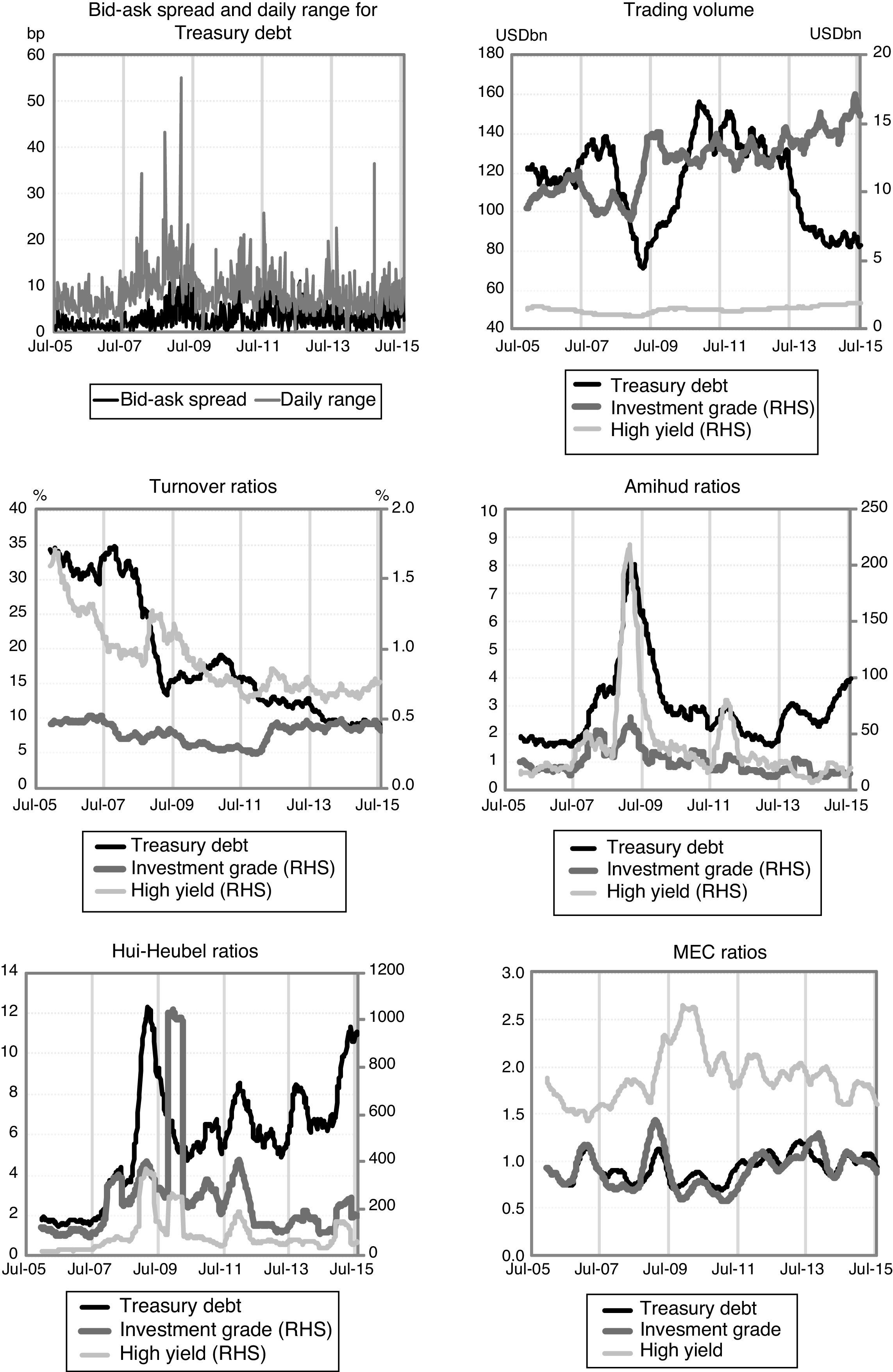
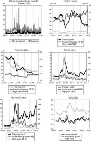
2.2

Individual market liquidity indicators for US fixed income markets

Fig. 1 reports the seventeen individual indicators, which depict a general worsening of liquidity conditions in US Treasury markets. The bid-ask spreads for US 10-y Treasury bond are wider than before the global financial crisis and spreads exhibit a more volatile pattern than in the past. This outcome is also evident in other metrics based on prices, such as the daily range. During 2015, trading volumes of long term government debt stood below USD 100 billion on a daily basis, below the figures recorded before the 2008 financial crisis of around USD 120. Moreover, the market size of long-term debt (7–11 years) has almost doubled since the onset of the crisis. Therefore, lower volumes have been accompanied by a sharp decline of the turnover rate, which in 2015 remained below 10%, significantly lower than the ratios of above 30% until 2007. The price impact indicators proposed by Amihud (2002) and by Hui and Heubel (1984) point to a reduced capacity of markets to minimize price movements under a certain flow of orders, as suggested by their upward trajectory since 2013. Finally, the MEC ratio suggests that resilience deteriorated during the 2008 crisis, but has recovered since then.

Fig. 1.

Individual market liquidity indicators for US fixed income markets. Note: Six-month averages except for the bid-ask spread and the daily range.

As shown in Fig. 1, in contrast to US government debt markets, the liquidity landscape for US corporate fixed income markets has been more benign.⁸ Due to data restrictions, for these markets we only compute five indicators, namely our volume-based measures and the MEC ratio. Trading volumes for both IG and HY markets have been raising steadily since 2009. Regarding HY debt, this increase has been smoother than that for debt outstanding, while for IG debt both measures have increased at a similar pace. Therefore, the turnover rate of HY debt has declined, whereas for IG markets it has maintained at pre-crisis levels (although in both cases the turnover ratios dropped below 1% in 2015). In contrast, the two price impact ratios for IG and HY markets have maintained levels rather similar to those prevailing before the crisis, although they exhibit some volatility spikes in the last half of the sample. Finally, the MEC ratio for HY debt basically has returned to pre-crisis levels after experiencing a sharp deterioration during the global financial crisis. Contrary to government debt, the MEC coefficient for HY debt is higher than one, which suggests lower market efficiency in this market.⁹

3

Methodology

3.1

Transformation of raw indicators

We want to represent overall liquidity conditions in US fixed income markets by means of an unique index. To this purpose, we construct an indicator so that an increase of its value reflects a worsening of market liquidity, whereas a decline of its value would suggest improving liquidity conditions. Therefore, all individual indicators should be transformed in order to reflect similar relations between their value and subsequent interpretation (i.e. higher value equals worsening conditions and vice versa). Out of the seventeen individual indexes, only for trading volumes and turnovers we need to use their inverse values instead in order to construct the index. Besides, in the case of the MEC ratios we use their absolute deviations from one, so that market resilience would increase under low values of this metric, and vice versa.

As our seventeen individual indicators are not homogeneous, we need to transform them to ensure methodological harmonization. One method that has been used traditionally in the literature of financial stress indicators is to normalize each variable using the mean and standard deviation. This approach has at least two caveats. First, it ignores the fact that each index has its own data scale, so standardized variables would not be comparable. Second, this standardization assumes that variables are normally distributed, which is usually not the case for financial variables (Holló et al., 2012). As a result, transformed variables are extremely sensitive to outliers, which may limit their informative value over time.

An alternative to normalization that overcomes these drawbacks is to transform each index alongside a common sample of the seventeen indicators by means of their empirical cumulative distribution function (CDF). This method has also been used, for instance, by the Federal Reserve Bank of Cleveland (Oet et al., 2011) to build its Financial Stress Index (FSI) or by Holló et al. (2012) to construct their Composite Indicator of Systemic Stress (CISS). The procedure is relatively straightforward. First, we order the values of our N = 17 indicators x_n, so that each indicator x = (x₁, x₂, …, x_T) with sample size T = 537 is transformed into its ordered sample (x_[1], x_[2], …, x_[T]). Hence, the lowest value of the indicator corresponds to x_[1] and the highest to x_[T]. If we denote r as the ranking number assigned to each value of x_t, the transformed liquidity indicators z_t computed from the empirical CDF would follow this expression,

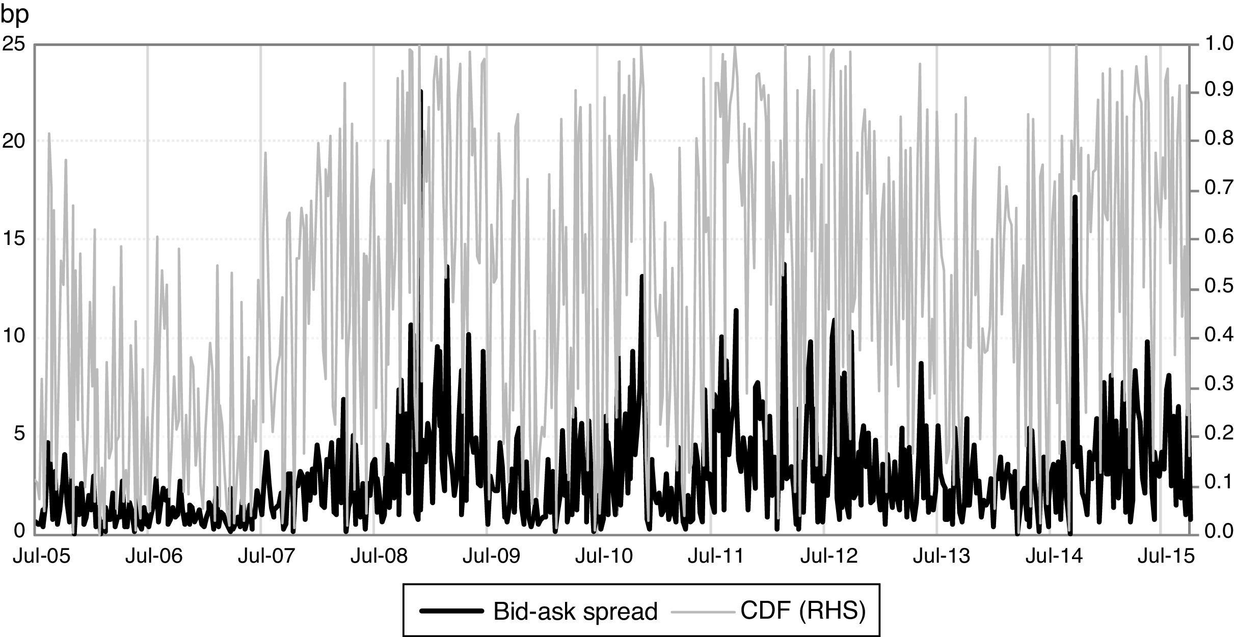
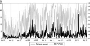
The CDF ensures that all indicators are bounded between 1/T and 1 for the whole sample period. Regarding repeated values, the function allocates to all of them their mean. By construction, once the CDF transformation is applied, the distance between two consecutive points is constrained to be 1/T. This implies a significant loss of information when analyzing the tails of the distributions, where the distance between two successive figures is wider. Nevertheless, this transformation reduces the sensitiveness of indicators to outliers and also increases the information content of points located around the mean of the distribution, which allows for the observation of early signals of tightening or loosening in the variables under study. The latter advantage is particularly relevant for timely policy assessments of changes in liquidity conditions. Fig. 2 illustrates these features of the transformation based on the CDF for the bid-ask spread of US Treasury bonds.

Fig. 2.

Bid-ask spread for US Treasury debt and associated transformation based on the CDF.

3.2

Aggregation

We aggregate the transformed liquidity variables into a single indicator by means of a principal component (PC) analysis. This approach converts the original variables (in our case the transformed liquidity measures) into uncorrelated PCs by a linear combination. The cumulative variance of the PCs equals the variance of the original variables; the first PC is the linear combination that represents the maximum variance of the original series.

The PC approach is a pure statistical procedure, with the limitation that our weights have no economic interpretation and do not take into account the theoretical importance of the original variables (OECD, 2008). Besides, the weights are constant over the whole sample so that interdependences among variables remain stable while in fact they may be changing (Oet et al., 2011). Finally, contrary to Holló et al. (2012), this procedure does not take into account the changing correlation between indicators throughout the sample, so that our synthetic indicator could overestimate liquidity tensions during normal times.

To overcome these problems, there are alternative methods to the PC analysis for the necessary aggregation of the values of the underlying indicators. These include the use of VAR models to account for the impact on a particular economic variable of interest of a set of financial indicators (Swiston, 2008) or the use of more sophisticated weighting schemes such as that in Holló et al. (2012) that takes into account the correlation structure of the original variables. In any case, we prefer the PC method as it is a well-known procedure that allows avoiding overlapping information between correlated indicators.

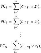
In our empirical exercise, we obtain N = 17 PCs that are linear combinations of the seventeen liquidity indicators.¹⁰

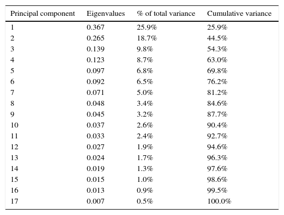
where a denotes the weights (also called components or factor loadings) assigned to the transformed indicators z in each PC.

As there is some degree of correlation between the original variables, there is a limited number of PCs that capture a major proportion of the total variance of the original series. In particular, as shown in Table 2, our first four PCs are able to explain over 60% of the original series’ variances. As we consider this figure a reasonable amount of information embedded in the original data, we choose these PCs and we extract their weights.

Table 2.

Eigenvalues extracted from the PCA procedure.

Principal component	Eigenvalues	% of total variance	Cumulative variance
1	0.367	25.9%	25.9%
2	0.265	18.7%	44.5%
3	0.139	9.8%	54.3%
4	0.123	8.7%	63.0%
5	0.097	6.8%	69.8%
6	0.092	6.5%	76.2%
7	0.071	5.0%	81.2%
8	0.048	3.4%	84.6%
9	0.045	3.2%	87.7%
10	0.037	2.6%	90.4%
11	0.033	2.4%	92.7%
12	0.027	1.9%	94.6%
13	0.024	1.7%	96.3%
14	0.019	1.3%	97.6%
15	0.015	1.0%	98.6%
16	0.013	0.9%	99.5%
17	0.007	0.5%	100.0%

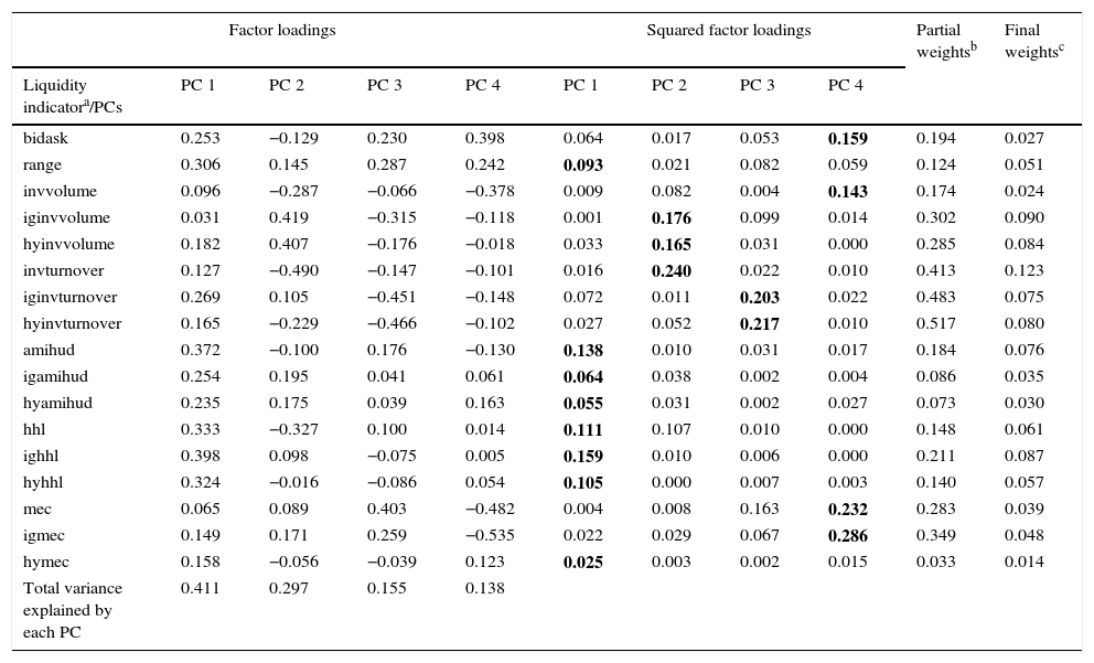
We follow the methodology of OECD (2008) to capture the information content of the four PCs in a unique vector of loadings. Following this approach, once we obtain the original factor loadings for the four PCs, we compute their squared values so that their sum is equal to one. Next, we construct an intermediate composite index in two steps. First, we select the highest factor loading for each of the seventeen indicators, and second, we compute the share of each one over the sum of the chosen factor loadings for each PC, so that the sum of these transformed weights is four, as the number of chosen PCs. Finally, we multiply these loadings by the proportion of the variance that each of the four PC explains, so that the new loadings add up to one. Table 3 reports the process followed to obtain the final weights.

Table 3.

Procedure to assign weights to individual indicators.

Factor loadings					Squared factor loadings				Partial weights^b	Final weights^c
Liquidity indicator^a/PCs	PC 1	PC 2	PC 3	PC 4	PC 1	PC 2	PC 3	PC 4
bidask	0.253	−0.129	0.230	0.398	0.064	0.017	0.053	0.159	0.194	0.027
range	0.306	0.145	0.287	0.242	0.093	0.021	0.082	0.059	0.124	0.051
invvolume	0.096	−0.287	−0.066	−0.378	0.009	0.082	0.004	0.143	0.174	0.024
iginvvolume	0.031	0.419	−0.315	−0.118	0.001	0.176	0.099	0.014	0.302	0.090
hyinvvolume	0.182	0.407	−0.176	−0.018	0.033	0.165	0.031	0.000	0.285	0.084
invturnover	0.127	−0.490	−0.147	−0.101	0.016	0.240	0.022	0.010	0.413	0.123
iginvturnover	0.269	0.105	−0.451	−0.148	0.072	0.011	0.203	0.022	0.483	0.075
hyinvturnover	0.165	−0.229	−0.466	−0.102	0.027	0.052	0.217	0.010	0.517	0.080
amihud	0.372	−0.100	0.176	−0.130	0.138	0.010	0.031	0.017	0.184	0.076
igamihud	0.254	0.195	0.041	0.061	0.064	0.038	0.002	0.004	0.086	0.035
hyamihud	0.235	0.175	0.039	0.163	0.055	0.031	0.002	0.027	0.073	0.030
hhl	0.333	−0.327	0.100	0.014	0.111	0.107	0.010	0.000	0.148	0.061
ighhl	0.398	0.098	−0.075	0.005	0.159	0.010	0.006	0.000	0.211	0.087
hyhhl	0.324	−0.016	−0.086	0.054	0.105	0.000	0.007	0.003	0.140	0.057
mec	0.065	0.089	0.403	−0.482	0.004	0.008	0.163	0.232	0.283	0.039
igmec	0.149	0.171	0.259	−0.535	0.022	0.029	0.067	0.286	0.349	0.048
hymec	0.158	−0.056	−0.039	0.123	0.025	0.003	0.002	0.015	0.033	0.014
Total variance explained by each PC	0.411	0.297	0.155	0.138

a

bidask = bid-ask spread; range = daily range; invvolume = 1/trading volume; invturnover = 1/turnover; amihud = Amihud ratio; hhl = Hui and Heubel ratio; mec = MEC ratio; “ig” and “hy” prefixes refer to investement grade and high yield indicators; PCs are the principal components.

b

Highest factor loadings in each indicator to the sum of factor loadings in bold in each PC.

c

Partial weights times percentage of variance in first four PCs explained by the correspondent PC.

4

Results

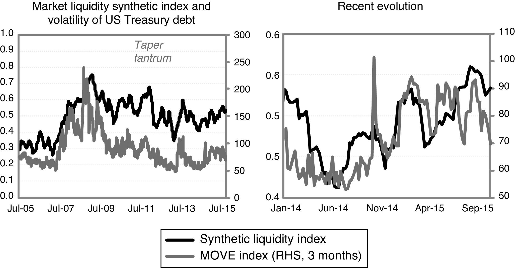
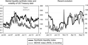
Fig. 3 displays the evolution of our synthetic market liquidity indicator. For the sake of comparability, the figure also shows the MOVE index, which is a widely used indicator that proxies tensions in fixed income markets.¹¹ As liquidity is an unobservable variable, we lack a proper benchmark to carry out a goodness-of-fit analysis. This problem is common to all synthetic liquidity indicators, but we mitigate this drawback by the comparison of our liquidity indicator with the MOVE index. In this, we make the implicit assumption that the MOVE is to some extent a suitable benchmark for liquidity conditions, i.e. movements in implicit volatilities in US Treasury bond markets reflect to a certain extent changing liquidity conditions in these markets.¹²

Fig. 3.

Market liquidity synthetic indicator (three-month averages) and MOVE index.

Market liquidity reached its low—that is, a maximum value of the indicator—during the global financial crisis at the end of 2008, amid a generalized volatility increase in international financial markets (see Fig. 3). After the crisis, the index exhibits two differentiated phases. First, until early 2013, liquidity gradually recovered, although it was still far from pre-crisis levels. The second period starts in mid-2013, during the so-called taper tantrum episode, when the index showed a spike. Once this turbulence episode was overcome, the indicator exhibited a continued deterioration of liquidity conditions. In both periods, bouts of increases in the liquidity indicator were accompanied by spikes in the MOVE index. At the same time, the former increases tended to reverse when volatility also faded. The strong correlation between both indicators suggests that our synthetic liquidity indicator at a minimum captures tensions in US fixed income markets as well.

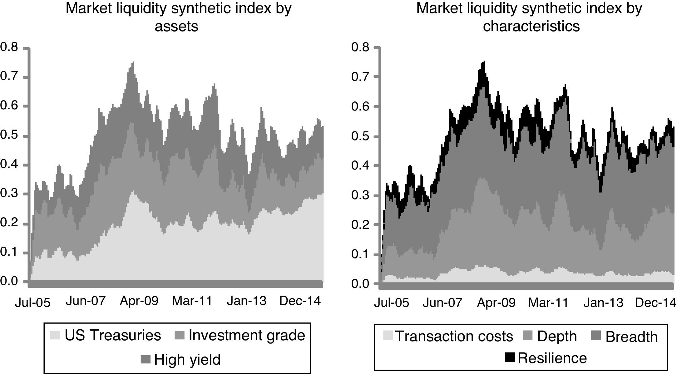
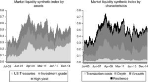
The index can be decomposed into two main categories, namely by asset type and by the liquidity characteristic covered by the individual indicators (Fig. 4). By asset type, developments in US Treasury bond markets have been mainly responsible for the deterioration in market liquidity that our index identifies after the taper tantrum episode. In contrast, liquidity in US corporate bond markets, which in principle are less liquid than US Treasury markets, has remained rather similar to that prevailing before the global financial crisis. We find similar results for both markets in the seventeen individual underlying liquidity metrics, but the reduction of the number of indicators in our synthetic index provides a simplified view that enhances data interpretation. Nevertheless, as mentioned before, the results for US corporate markets need to be carefully interpreted, as they are based on indexes obtained from a basket of thousands of bonds that might be quite heterogeneous in nature.

Fig. 4.

Market liquidity synthetic indicator by asset and by characteristic of the individual indicators.

With regard to liquidity characteristics, indicators that represent depth and breadth are responsible for most of the deterioration in liquidity. That is, the indicators measuring the number of transactions (volume based measures) and the price sensitivity of bonds to the traded volume (price impact ratios), respectively, capture most of the dynamics of the synthetic index. The resilience of fixed income markets, that is, the ease with which prices move towards their theoretical values of equilibrium, has also been eroded since mid-2013. Finally, the contribution of transaction costs to the index remains stable across the sample, which supports the hypothesis that indicators such as the bid-ask spread are a poor proxy of overall market liquidity conditions (Bao et al., 2011; IMF, 2015).

5

Conclusions

In this paper, we study liquidity conditions in US fixed income markets through a new synthetic index based on seventeen individual indicators for both government and corporate debt. The approach that we follow to construct the index consist of two steps. First, we transform the original variables using the cumulative distribution function, so that they are rescaled homogeneously, while reducing their sensitiveness to outliers. Second, we aggregate the transformed variables following a PC-based procedure that prevents information provided by the original indicators to overlap with each other. The synthetic index reflects deteriorating liquidity conditions when compared with those prevailing before the global financial crisis as well as increasing tensions in market liquidity from mid-2013 to late 2015. By asset class, liquidity in US Treasury bond markets has deteriorated, whereas that in US corporate bond markets has been more stable. By individual liquidity indicator, price impact ratios have been the most severely affected after the crisis and hence have been the main driver of the increase in our synthetic index.

Finally, there are several issues that have not been addressed in this paper, which could serve as lines for future research. First, the procedure to obtain the index could be implemented in a recursive way, as in Holló et al. (2012). Second, we could enhance the aggregation method by considering the correlations among the individual indices. Third, we have not investigated in detail the relationship between market liquidity and market volatility. Given the lack of a proper liquidity benchmark, further analysis on the link between both variables would deserve further research.