

We evaluated the relevance of threshold selection in species distribution models on the delimitation of areas of endemism, using as case study the North American mammals. We modeled 40 species of endemic mammals of the Nearctic region with Maxent, and transformed these models to binary maps using four different thresholds: minimum training presence, tenth percentile training presence, equal training sensitivity and specificity, and 0.5 logistic probability. We analyzed the binary maps with the optimality method in order to identify areas of endemism and compare our results regarding previous analyses. The majority of the species tend to have very low values for the minimum training presence, whereas most of the species have a value of the tenth percentile training presence around 0.5, and the equal training sensitivity and specificity was around 0.3. Only with the tenth percentile threshold we recovered three out of the four patterns of endemism identified in North America, and detected more endemic species.The best identification of areas of endemism was obtained using the tenth percentile training presence threshold, which seems to recover better the distributional area of the mammals analyzed.
Evaluamos la relevancia de la selección del umbral en los modelos de distribución de especies en la delimitación de las áreas de endemismo, usando como un caso de estudio a los mamíferos de América del Norte. Modelamos 40 especies de mamíferos endémicos de la región Neártica con Maxent, y transformamos esos modelos a mapas binarios usando cuatro umbrales diferentes: presencia mínima de entrenamiento, percentil diez de la presencia de entrenamiento, igual sensibilidad y especificidad de entrenamiento, y probabilidad logística de 0.5. Los mapas binarios los analizamos con el método de optimación con el objeto de identificar áreas de endemismo y comparar nuestros resultados con estudios previos. La mayoría de las especies mostró tendencias hacia valores muy bajos de la presencia mínima de entrenamiento, mientras que la mayoría tuvo un valor del percentil diez de la presencia de entrenamiento alrededor de 0.5, y de igual sensibilidad y especificidad de entrenamiento alrededor de 0.3. Únicamente con el percentil diez de la presencia de entrenamiento se recuperaron tres de los cuatro patrones de endemismo identificados para América del Norte y se detectaron más especies endémicas. La identificación de áreas de endemismo más eficiente se obtuvo usando el umbral del percentil diez de la presencia de entrenamiento, el cual parece recuperar mejor las áreas de distribución de los mamíferos analizados.
Species distribution models (also named ecological niche models) are commonly used in biogeography. In particular, although they are more suited for the identification of ecological biogeographical patterns, they also have important applications in the identification of historical biogeographical patterns, namely, generalized tracks1 and areas of endemism2-6 where models have been used to improve their delimitation.
There are many modeling techniques (GLM, GAM, GARP, ENFA, Maxent, etc.), which can be used depending on the available records (data) for each species, environmental data and the required accuracy of the models. Some comparisons of the different modeling techniques have been performed7-9 and although there are no general conclusions, Maxent10-12 seems to perform better than others. Maxent generates probability maps of species presence in three output formats: raw, cumulative and logistic (see Maxent tutorial, http://www.cs.princeton.edu/~schapire/maxent/), being the last two the most used (in scales of 0-100 and 0-1, respectively).
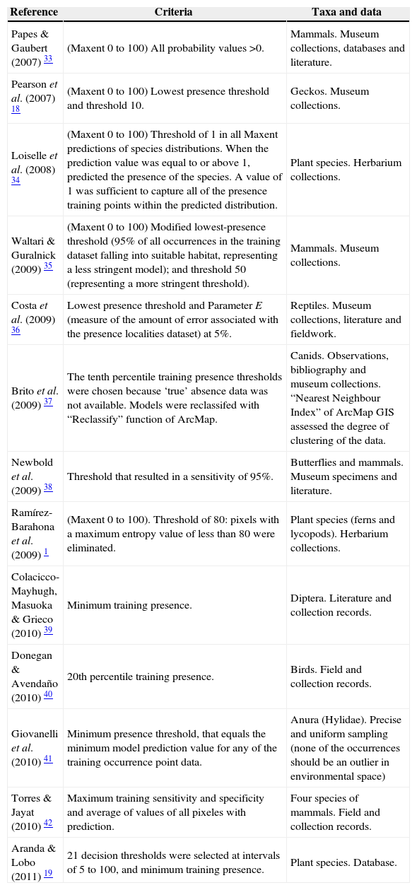
As in conservation and environmental management practices13, in biogeography sometimes it is necessary to transform probabilistic data to presence/absence data (binary maps, i.e. 1 - 0). For this to be feasible, a probability threshold has to be established to the minimun level at which the distributions should be left out. As there are many possible uses for distribution models, some methods have been proposed in order to select the best threshold in Maxent to obtain a binary map for species (see Table I). They include the minimum (or lowest) training presence, threshold of a particular percentage (10, 50, 80%), sensitivity at 95%, some percentile training presence (10, 20), equal training sensitivity and specificity, etc. (Pawar et al.14 for further details). However, there has been some comparisons and evaluations that might allow to select the best threshold for other modeling algorithms generally related with prevalence, sensitivity and specificity13,15-17, and specifically for Maxent18-20 (see Table I). So, there is not a consensus about which is the way to select the best threshold.
Some thresholds for Maxent to transform to binary maps, using different taxa and origin of data. For the criteria described in this table, sensitivity refers to the proportion of presences correctly predicted. Specificity is the proportion of abscences correctly predicted. Both are indices, not criteria. Prevalence refers to the proportion of the study area covered by the species’ distributional area13.
| Reference | Criteria | Taxa and data |
|---|---|---|
| Papes & Gaubert (2007) 33 | (Maxent 0 to 100) All probability values >0. | Mammals. Museum collections, databases and literature. |
| Pearson et al. (2007) 18 | (Maxent 0 to 100) Lowest presence threshold and threshold 10. | Geckos. Museum collections. |
| Loiselle et al. (2008) 34 | (Maxent 0 to 100) Threshold of 1 in all Maxent predictions of species distributions. When the prediction value was equal to or above 1, predicted the presence of the species. A value of 1 was sufficient to capture all of the presence training points within the predicted distribution. | Plant species. Herbarium collections. |
| Waltari & Guralnick (2009) 35 | (Maxent 0 to 100) Modified lowest-presence threshold (95% of all occurrences in the training dataset falling into suitable habitat, representing a less stringent model); and threshold 50 (representing a more stringent threshold). | Mammals. Museum collections. |
| Costa et al. (2009) 36 | Lowest presence threshold and Parameter E (measure of the amount of error associated with the presence localities dataset) at 5%. | Reptiles. Museum collections, literature and fieldwork. |
| Brito et al. (2009) 37 | The tenth percentile training presence thresholds were chosen because ‘true’ absence data was not available. Models were reclassifed with “Reclassify” function of ArcMap. | Canids. Observations, bibliography and museum collections. “Nearest Neighbour Index” of ArcMap GIS assessed the degree of clustering of the data. |
| Newbold et al. (2009) 38 | Threshold that resulted in a sensitivity of 95%. | Butterflies and mammals. Museum specimens and literature. |
| Ramírez-Barahona et al. (2009) 1 | (Maxent 0 to 100). Threshold of 80: pixels with a maximum entropy value of less than 80 were eliminated. | Plant species (ferns and lycopods). Herbarium collections. |
| Colacicco-Mayhugh, Masuoka & Grieco (2010) 39 | Minimum training presence. | Diptera. Literature and collection records. |
| Donegan & Avendaño (2010) 40 | 20th percentile training presence. | Birds. Field and collection records. |
| Giovanelli et al. (2010) 41 | Minimum presence threshold, that equals the minimum model prediction value for any of the training occurrence point data. | Anura (Hylidae). Precise and uniform sampling (none of the occurrences should be an outlier in environmental space) |
| Torres & Jayat (2010) 42 | Maximum training sensitivity and specificity and average of values of all pixeles with prediction. | Four species of mammals. Field and collection records. |
| Aranda & Lobo (2011) 19 | 21 decision thresholds were selected at intervals of 5 to 100, and minimum training presence. | Plant species. Database. |
Areas of endemism are basic biogeographic units, their identification is the first step of an evolutionary biogeographic analysis and they are a pre-requisite of any cladistic biogeographic analysis21. An area of endemism is an area of non-random distributional congruence of two or more taxa22, and the basis of biogeographic regionalizations23. The identification of areas of endemism depends totally on maps of distribution of species and their generalization to spatial units. The most used units of study are grid-cells, although it is possible to use other regular polygons or even polygons with irregular forms. The most popular methods (Parsimony Analysis of Endemicity21 and Endemicity analysis24,25) employ data matrices of presence/absence of species in quadrats. Thus, the identification of areas of endemism can be affected by the generalization of individual areas of distribution to the grid-cells. Some authors6,26 pointed that the use of species distribution models (or ecological niche models) can modify the identification of areas of endemism due to the overprediction involved in them; however, this has not been proved.
Escalante et al.27 recently published a study of identification of Nearctic areas of endemism using mammals. They used areas of distribution drawn by traditional methodology (areas inferred by mammalogists specialists; maps available on http://conabioweb.conabio.gob.mx/website/mamiferos/viewer.htm28), in order to analyze the main patterns of endemism corresponding to the Nearctic region. They obtained four areas in North America identified by 40 species: Nearctic, Western, Eastern and Northern patterns.
We evaluate herein the relevance of the selection of the threshold in Maxent using four different options (minimum training presence, tenth percentile training presence, equal training sensitivity and specificity and 0.5 logistic probability), and its impact on the delimitation of areas of endemism, using as study case the mammals of the Nearctic region.
Material and methodsWe compiled a database of 40 species of endemic mammals of North America (following Escalante et al.27) corresponding to five orders (Table II). Those species gave score to some area of endemism in that publication, and shown sympatric patterns. Records were obtained from a database of mammals of Mexico (Mammex; Escalante et al., unpublished data), and four on-line databases: GBIF (http://www.gbif.org/), MaNIS (http://manisnet.org/), CONABIO (Remib; http://www.conabio.gob.mx/), and UNIBIO (Instituto de Biología, UNAM; http://unibio.ibiologia.unam.mx/). A record is considered as a unique combination of the name of the species and georreferenced site (latitude-longitude) (Table II). Localities of each species were geographically validated in a Geographic Information System (GIS; ArcGis 9.3)29, using specialized bibliography30,31 and two websites: North American Mammals (http://www.mnh.si.edu/mna/) and Infonatura (http://www.natureserve.org/infonatura/).
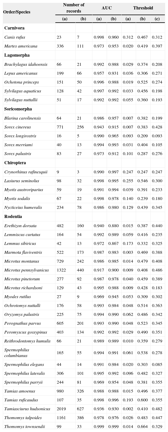
Data of the models for endemic species. Number of records: (a) used in the training of models and (b) in the test of models; the AUC for: (a) training and (b) testing; and the value of the threshold for logistic models: (a) minimum training presence, and (b) the tenth percentile training presence, and (c) equal training sensitivity and specificity.
| Order/Species | Number of records | AUC | Threshold | ||||
|---|---|---|---|---|---|---|---|
| (a) | (b) | (a) | (b) | (a) | (b) | (c) | |
| Carnivora | |||||||
| Canis rufus | 23 | 7 | 0.998 | 0.960 | 0.312 | 0.467 | 0.312 |
| Martes americana | 336 | 111 | 0.973 | 0.953 | 0.020 | 0.419 | 0.397 |
| Lagomorpha | |||||||
| Brachylagus idahoensis | 66 | 21 | 0.992 | 0.988 | 0.029 | 0.374 | 0.208 |
| Lepus americanus | 199 | 66 | 0.957 | 0.931 | 0.036 | 0.306 | 0.271 |
| Ochotona princeps | 151 | 50 | 0.996 | 0.988 | 0.019 | 0.525 | 0.274 |
| Sylvilagus aquaticus | 128 | 42 | 0.997 | 0.992 | 0.033 | 0.456 | 0.198 |
| Sylvilagus nuttallii | 51 | 17 | 0.992 | 0.992 | 0.055 | 0.360 | 0.193 |
| Soricomorpha | |||||||
| Blarina carolinensis | 64 | 21 | 0.986 | 0.957 | 0.007 | 0.382 | 0.199 |
| Sorex cinereus | 771 | 256 | 0.943 | 0.915 | 0.007 | 0.383 | 0.428 |
| Sorex longirostris | 16 | 5 | 0.990 | 0.965 | 0.093 | 0.209 | 0.093 |
| Sorex merriami | 40 | 13 | 0.994 | 0.993 | 0.031 | 0.404 | 0.105 |
| Sorex palustris | 83 | 27 | 0.973 | 0.912 | 0.101 | 0.287 | 0.276 |
| Chiroptera | |||||||
| Crynorhinus rafinesquii | 9 | 3 | 0.990 | 0.997 | 0.247 | 0.247 | 0.247 |
| Lasiurus seminolus | 98 | 32 | 0.998 | 0.995 | 0.255 | 0.546 | 0.300 |
| Myotis austroriparius | 59 | 19 | 0.991 | 0.994 | 0.039 | 0.391 | 0.233 |
| Myotis sodalis | 67 | 22 | 0.998 | 0.978 | 0.140 | 0.239 | 0.180 |
| Nycticeius humeralis | 234 | 78 | 0.986 | 0.980 | 0.129 | 0.439 | 0.345 |
| Rodentia | |||||||
| Erethizon dorsata | 482 | 160 | 0.940 | 0.880 | 0.015 | 0.387 | 0.440 |
| Lemmiscus curtatus | 164 | 54 | 0.992 | 0.989 | 0.059 | 0.416 | 0.235 |
| Lemmus sibiricus | 42 | 13 | 0.972 | 0.867 | 0.173 | 0.332 | 0.325 |
| Marmota flaviventris | 522 | 173 | 0.987 | 0.983 | 0.003 | 0.469 | 0.388 |
| Microtus montanus | 729 | 242 | 0.986 | 0.985 | 0.014 | 0.479 | 0.408 |
| Microtus pennsylvanicus | 1322 | 440 | 0.917 | 0.900 | 0.009 | 0.408 | 0.486 |
| Microtus pinetorum | 277 | 92 | 0.987 | 0.978 | 0.040 | 0.459 | 0.389 |
| Microtus richardsoni | 129 | 43 | 0.995 | 0.988 | 0.009 | 0.428 | 0.183 |
| Myodes rutilus | 27 | 9 | 0.969 | 0.945 | 0.053 | 0.309 | 0.302 |
| Ochrotomys nuttalli | 176 | 58 | 0.993 | 0.984 | 0.048 | 0.514 | 0.363 |
| Oryzomys palustris | 225 | 75 | 0.994 | 0.990 | 0.062 | 0.486 | 0.342 |
| Perognathus parvus | 605 | 201 | 0.993 | 0.990 | 0.048 | 0.523 | 0.345 |
| Peromyscus gossypinus | 403 | 134 | 0.992 | 0.992 | 0.029 | 0.490 | 0.351 |
| Reithrodontomys humulis | 66 | 21 | 0.989 | 0.989 | 0.010 | 0.359 | 0.279 |
| Spermophilus columbianus | 165 | 55 | 0.994 | 0.991 | 0.061 | 0.538 | 0.278 |
| Spermophilus elegans | 44 | 14 | 0.991 | 0.984 | 0.020 | 0.303 | 0.085 |
| Spermophilus lateralis | 306 | 101 | 0.995 | 0.992 | 0.096 | 0.482 | 0.327 |
| Spermophilus parryii | 244 | 81 | 0.969 | 0.954 | 0.048 | 0.381 | 0.355 |
| Tamias amoenus | 980 | 326 | 0.988 | 0.988 | 0.015 | 0.496 | 0.377 |
| Tamias ruficaudus | 107 | 35 | 0.998 | 0.996 | 0.193 | 0.600 | 0.355 |
| Tamiasciurus hudsonicus | 2019 | 627 | 0.936 | 0.930 | 0.002 | 0.410 | 0.482 |
| Thomomys talpoides | 1161 | 386 | 0.978 | 0.976 | 0.026 | 0.483 | 0.447 |
| Thomomys townsendii | 99 | 33 | 0.999 | 0.999 | 0.014 | 0.664 | 0.329 |
To construct the models in Maxent, 23 environmental data layers were used at a resolution of ~2 km (which is suitable for our study area): four topographic layers were obtained from Hydro1k (http://edc.usgs.gov/products/elevation/gtopo30/hydro/namerica.html) while 19 climatic data layers were derived from the WorldClim database (http://www.worldclim.org/32: altitude, aspect, compound topographic index, slope, annual mean temperature, mean diurnal range, isothermality, temperature seasonality, maximum temperature of warmest month, minimum temperature of coldest month, temperature annual range, mean temperature of wettest quarter, mean temperature of driest quarter, mean temperature of warmest quarter, mean temperature of coldest quarter, annual precipitation, precipitation of wettest month, precipitation of driest month, precipitation seasonality, precipitation of wettest quarter, precipitation of driest quarter, precipitation of warmest quarter and precipitation of coldest quarter.
For each species, 25% of the records were used to validate the model internally. The algorithm of Maxent uses a series of rules to calculate probabilities. For the present analysis, all rules were used, so the program selects the adequate one depending on the number of available data. The used rules are: (a) linear, which uses the variable by itself; (b) quadratic, which uses the square of the variable; (c) product, which uses the product of two variables; (d) threshold, which uses a binary transformation (0, 1) of a continuous variable using a threshold; and (e) hinge, which is like the lineal rule, but remains constant under the threshold. The algorithm determines which rule to use like follows: lineal if there are < 10 points; lineal + cuadratic if there are 10-14 points; lineal + cuadratic + hinge if there are 15-79 points; and all if there are > 80 points (http://www.cs.princeton.edu/~schapire/maxent/tutorial/tutorial.doc). The logistic value output was selected because is the easiest to conceptualize since it gives an estimate between 0 and 1 of probability of presence (see http://www.cs.princeton.edu/~schapire/maxent/tutorial/tutorial.doc for further details).
Model success was judged using two criteria: AUC > 0.7, and p < 0.05 for at least one binomial test14, and both obtained from the program. AUC, or area under the curve, is an index used to evaluate models because it provides a single measure of overall accuracy that is not dependent upon a particular threshold43. The value of the AUC ranges between 0 and 1.0. Values of 0.5 implies that the scores for two groups (random and model) do not differ, while a score of 1.0 indicates no overlap in the distributions, and the model is reliable. A value of 0.8 for the AUC means that for 80% of the time a random selection from the positive group will have a score greater than a random selection from the negative class. It is important to note that AUC values tend to be higher for species with narrow ranges, relative to the study area described by the environmental data. This does not necessarily mean that the models are better; instead this behavior is an artifact of the AUC statistic43.
Models were generated in ascii format, and exported directly to the GIS.We selected four of the most common used thresholds for Maxent models in logistic format: the minimum training presence, the tenth percentile training presence, the equal training sensitivity and specificity (obtained from the output table of Maxent), and a logistic probability of 0.5. All pixels with a value under those thresholds were assigned a value of zero (0), which would represent absence of the species.
To analyze the influence of the four thresholds on the delimitation of areas of endemism, the 40 endemic species were analyzed, in order to prove if we identify the patterns previously discovered27. We overlapped and intersected the binary maps obtained for each species, using each one of the four thresholds (minimum training presence, tenth percentile training presence, equal training sensitivity and specificity and logistic probability of 0.5) to a 4º latitude-longitude grid. Then, we built four matrices of presence/absence (one for each threshold), where the predicted presence of a species was coded as “1” and its absence was coded as “0”. We performed four analysis of endemicity with the optimality method24,25, one for each threshold. The optimality method calculates a score of endemicity for a taxon to a given area (grid), so, the endemicity for an area will be the sum of the scores of two or more taxa inhabitting it. From among different possible areas, those with the highest scores of endemicity are preferred.
The four analyses of endemicity were developed in NDM/ VNDM v. 2.544 (available at www.zmuc.dk/public/phylogeny), where each matrix was analyzed iteratively changing the random seed until the number of areas of endemism remained stable. We used the same parameters used by Escalante et al.27: heuristic search saving sets of areas with two or more endemic species, save sets with score above 2, and optimal sets were chosen when having above 50% of different endemic species to the highest score. When we obtained two or more areas of endemism, consensus areas were calculated using 30% of similarity in species against any of the other areas in the consensus. We obtained the number of endemic taxa of each matrix and their consensus areas of endemism. All areas of endemism were analyzed regarding their scores, patterns represented and number of endemic species, in order to compare them with the analysis of Escalante et al.27 and to evaluate the performance of the four thresholds.
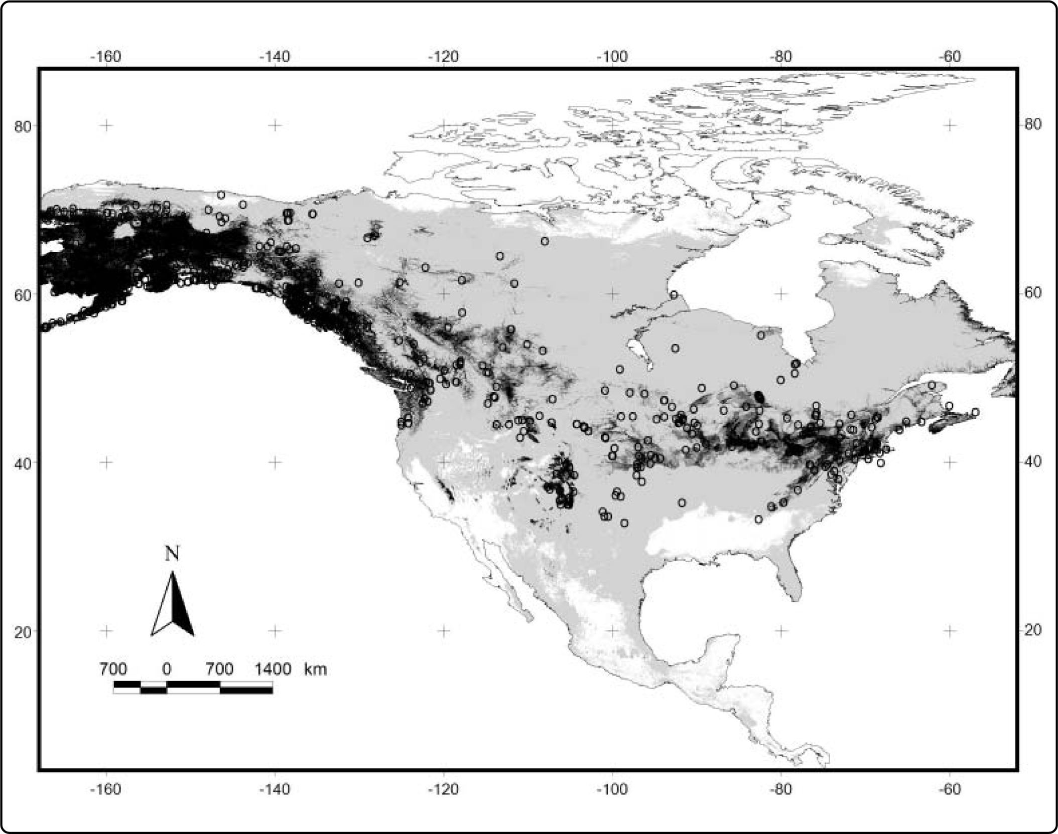
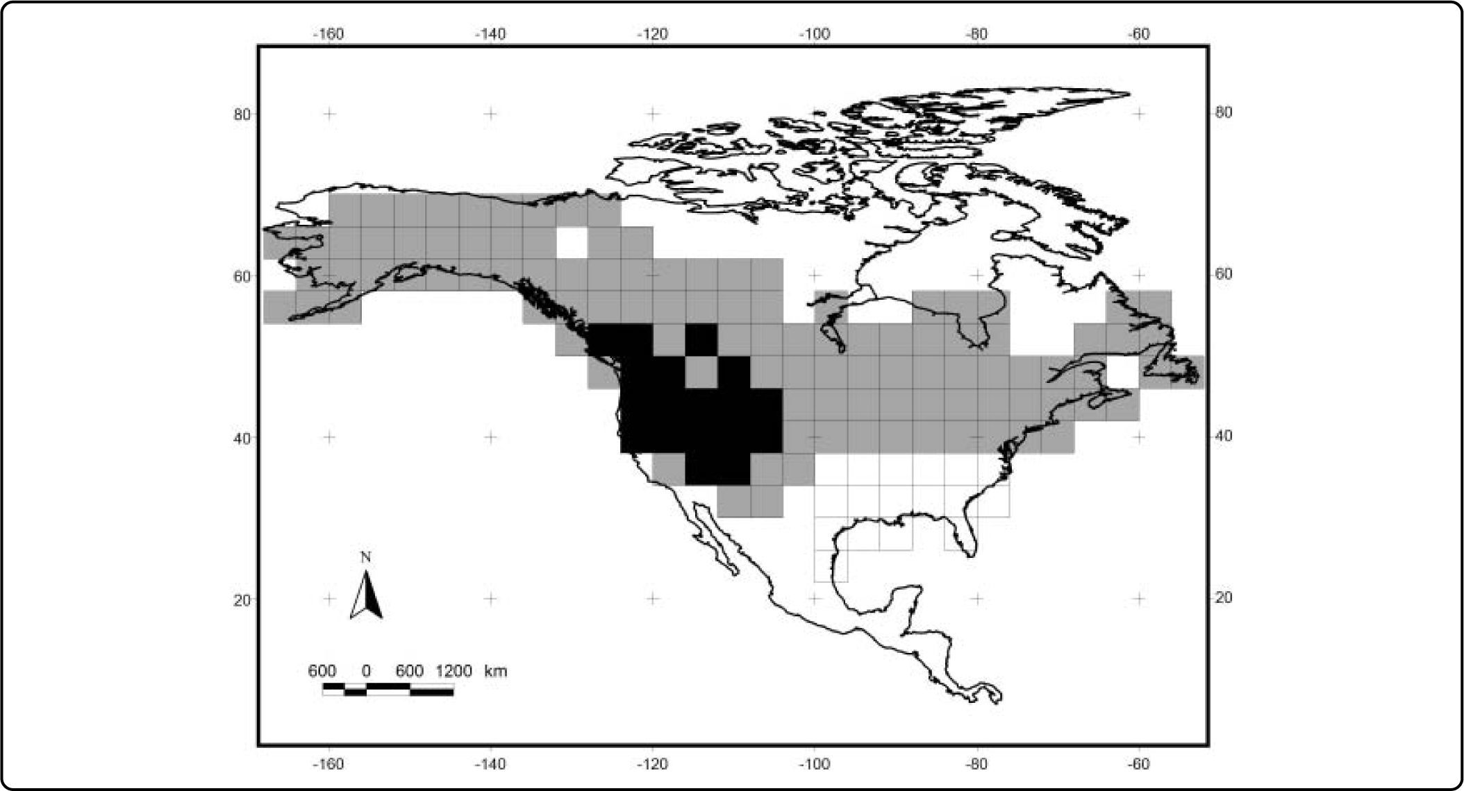
ResultsWe obtained 40 models from Maxent (one for each species). The average value for the AUC for training was 0.98 and 0.96 for testing (see Table II). The values for the minimum training presence, the tenth percentile training presence and the equal training sensitivity and specificity thresholds for each species are shown in Table II. The range for the minimum training presence was 0.002 - 0.312, for the tenth percentile presence was 0.209 - 0.664, and for the equal training sensitivity and specificity was 0.085-0.486, with averages of 0.065, 0.412, and 0.303, respectively. Most of the species tend to have very low values for the minimum training presence, whereas most of species have a value of the tenth percentile training presence around of 0.5, and the equal training sensitivity and specificity less than 0.5. An example of the differences between the binary maps resulting form the application of four thresholds is shown in Figures 1 and 2.
; medium gray, the equal training sensitivity and specificity (0.428); and light gray, the minimum training presence (0.007). Circles: data points.")
Map of potential distribution of Sorex cinereus in North America with four different thresholds: black, the probability of 0.5; dark gray, the tenth percentile training presence (0.383); medium gray, the equal training sensitivity and specificity (0.428); and light gray, the minimum training presence (0.007). Circles: data points.
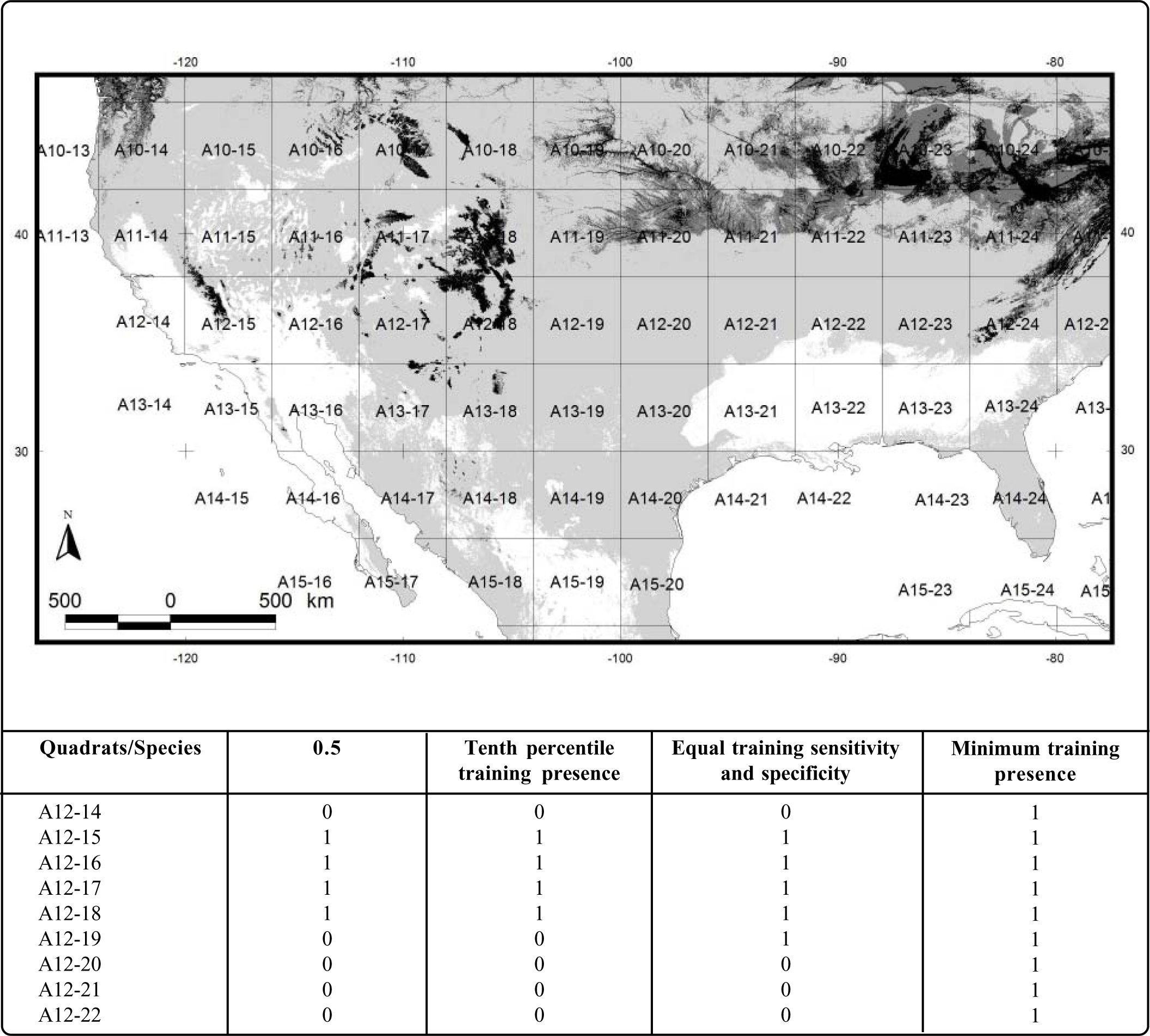
; medium gray: the equal training sensitivity and specificity (0.428); and light gray: the minimum training presence (0.007).")
Detail of a generalization of the four potential distributional areas of Sorex cinereus to a 4º grid on the Mexico-U.S.A border. The presence predicted by each map in a quadrat is coded with “1”, and the absence with “0”. The label of each 4º quadrat is showed as A#-#. Black: the probability of 0.5; dark gray: the tenth percentile training presence (0.383); medium gray: the equal training sensitivity and specificity (0.428); and light gray: the minimum training presence (0.007).
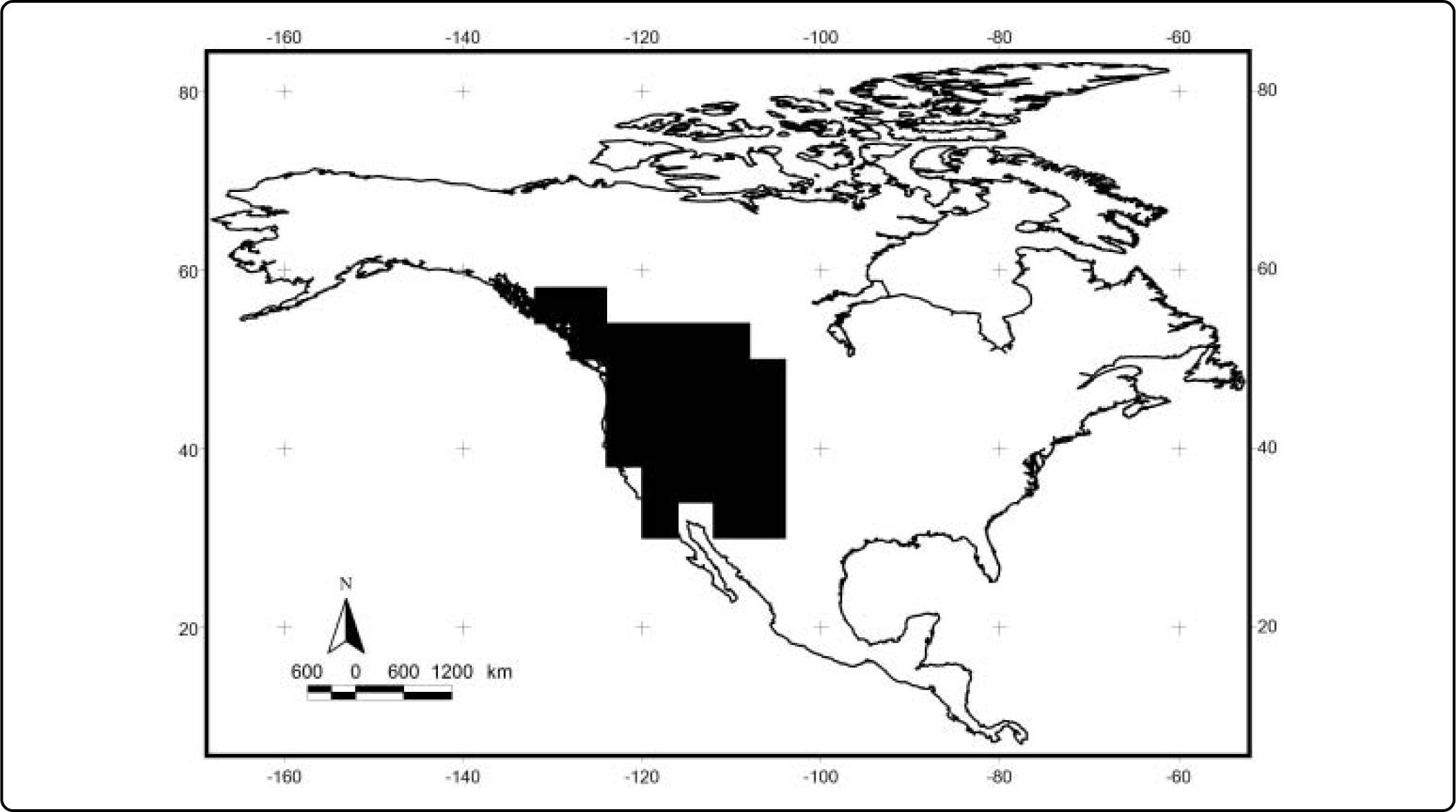
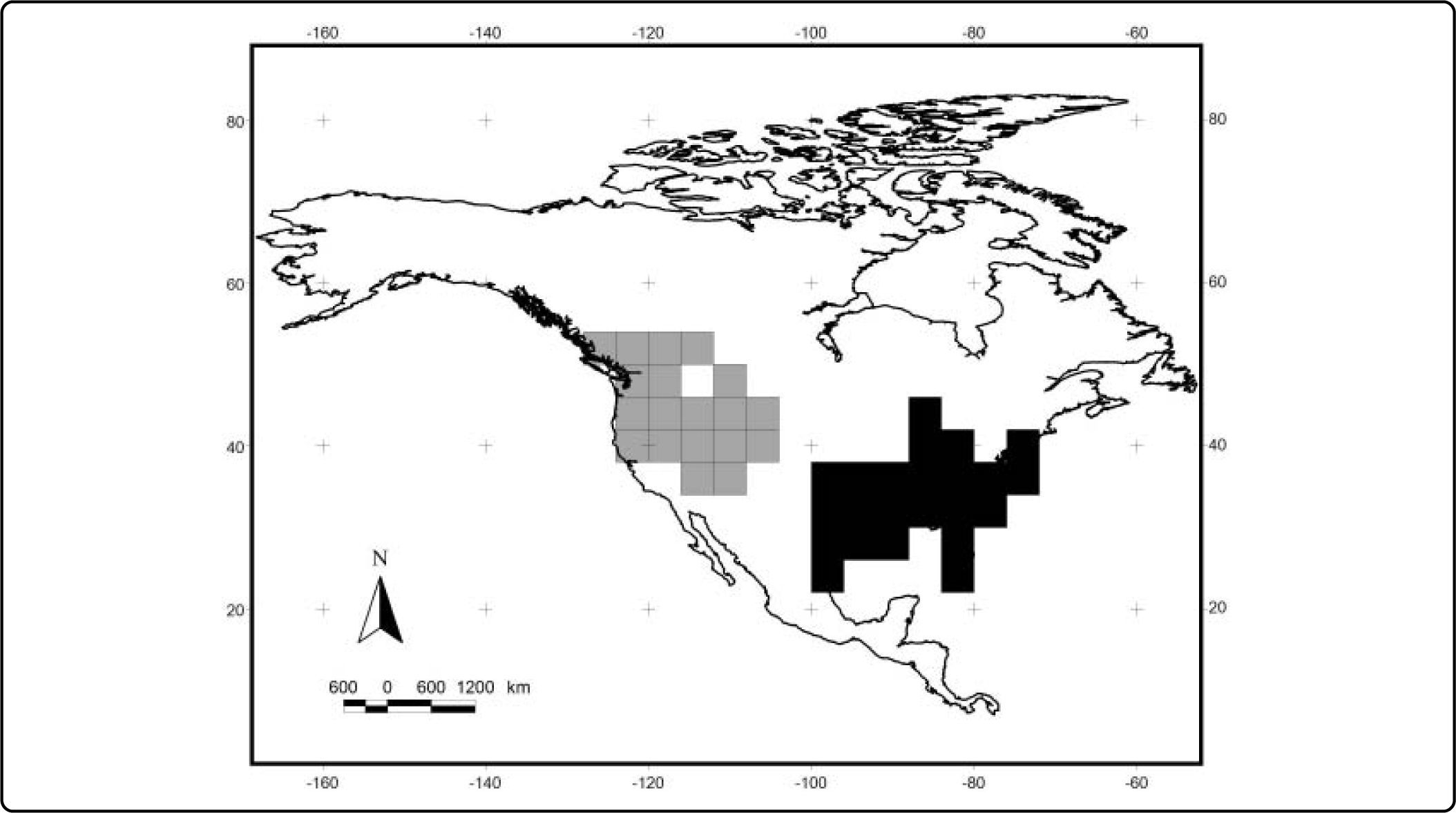
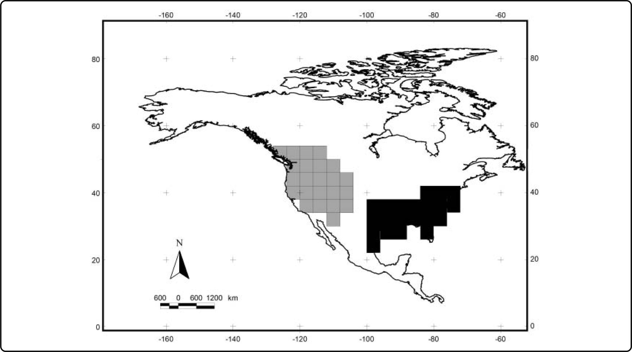
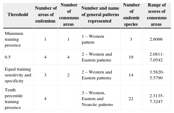
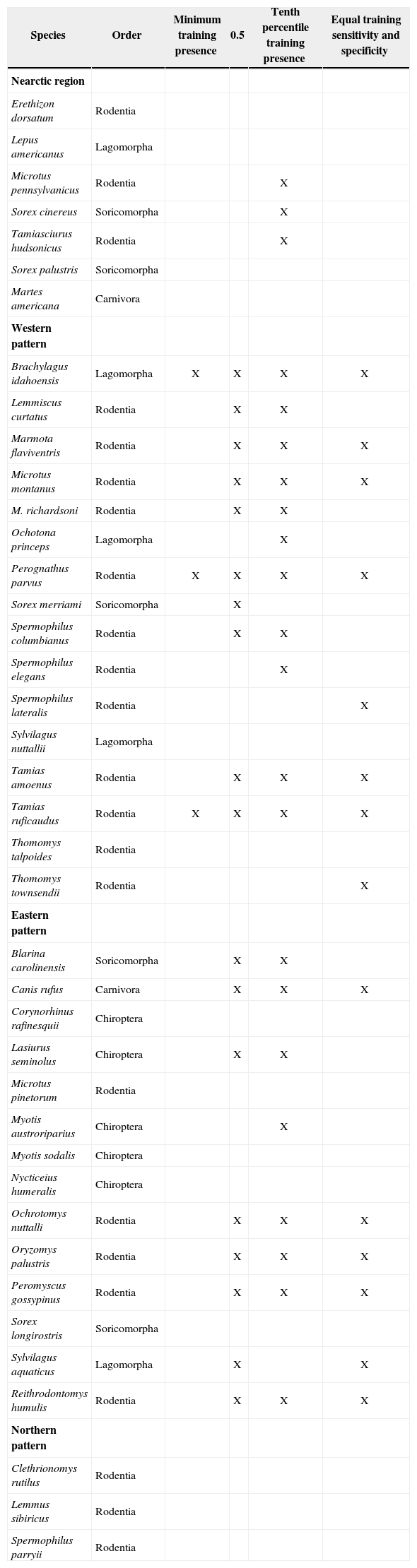
The results of the analyses of endemicity are shown in Tables III and IV. In the analysis using the minimum training presence threshold, we could recover only one pattern of endemism (Fig. 3): the Western pattern of Escalante et al.27 With the tenth percentile threshold we recovered three patterns (Fig. 4): Nearctic, Western and Eastern; with the 0.5 value of probability as a threshold, we recovered two patterns (Fig. 5): Western and Eastern; and the same with the equal training sensitivity and specificity, two patterns were identified: Western and Eastern (Fig. 6). Moreover, the threshold where we obtained more endemic species was the tenth percentile, followed by the 0.5, the equal training sensitivity and specificity and the minimum training presence (Table IV). Only one pattern (the Northern pattern) of Escalante et al.27 could not be recovered with any of the thresholds.
Areas of endemism and consensus areas for each threshold.
| Threshold | Number of areas of endemism | Number of consensus areas | Number and name of general patterns represented | Number of endemic species | Range of scores of consensus areas |
|---|---|---|---|---|---|
| Minimum training presence | 1 | 1 | 1 – Western pattern | 3 | 2.6096 |
| 0.5 | 4 | 4 | 2 – Western and Eastern patterns | 19 | 2.0811-7.0542 |
| Equal training sensitivity and specificity | 3 | 2 | 2 – Western and Eastern patterns | 14 | 3.5820-5.5790 |
| Tenth percentile training presence | 4 | 3 – Western, Eastern and Nearctic patterns | 22 | 2.3135-7.3247 |
Results of the analyses of endemicity for 40 endemic species of the Nearctic region for three thresholds. X= species recovered in each analysis.
| Species | Order | Minimum training presence | 0.5 | Tenth percentile training presence | Equal training sensitivity and specificity |
|---|---|---|---|---|---|
| Nearctic region | |||||
| Erethizon dorsatum | Rodentia | ||||
| Lepus americanus | Lagomorpha | ||||
| Microtus pennsylvanicus | Rodentia | X | |||
| Sorex cinereus | Soricomorpha | X | |||
| Tamiasciurus hudsonicus | Rodentia | X | |||
| Sorex palustris | Soricomorpha | ||||
| Martes americana | Carnivora | ||||
| Western pattern | |||||
| Brachylagus idahoensis | Lagomorpha | X | X | X | X |
| Lemmiscus curtatus | Rodentia | X | X | ||
| Marmota flaviventris | Rodentia | X | X | X | |
| Microtus montanus | Rodentia | X | X | X | |
| M. richardsoni | Rodentia | X | X | ||
| Ochotona princeps | Lagomorpha | X | |||
| Perognathus parvus | Rodentia | X | X | X | X |
| Sorex merriami | Soricomorpha | X | |||
| Spermophilus columbianus | Rodentia | X | X | ||
| Spermophilus elegans | Rodentia | X | |||
| Spermophilus lateralis | Rodentia | X | |||
| Sylvilagus nuttallii | Lagomorpha | ||||
| Tamias amoenus | Rodentia | X | X | X | |
| Tamias ruficaudus | Rodentia | X | X | X | X |
| Thomomys talpoides | Rodentia | ||||
| Thomomys townsendii | Rodentia | X | |||
| Eastern pattern | |||||
| Blarina carolinensis | Soricomorpha | X | X | ||
| Canis rufus | Carnivora | X | X | X | |
| Corynorhinus rafinesquii | Chiroptera | ||||
| Lasiurus seminolus | Chiroptera | X | X | ||
| Microtus pinetorum | Rodentia | ||||
| Myotis austroriparius | Chiroptera | X | |||
| Myotis sodalis | Chiroptera | ||||
| Nycticeius humeralis | Chiroptera | ||||
| Ochrotomys nuttalli | Rodentia | X | X | X | |
| Oryzomys palustris | Rodentia | X | X | X | |
| Peromyscus gossypinus | Rodentia | X | X | X | |
| Sorex longirostris | Soricomorpha | ||||
| Sylvilagus aquaticus | Lagomorpha | X | X | ||
| Reithrodontomys humulis | Rodentia | X | X | X | |
| Northern pattern | |||||
| Clethrionomys rutilus | Rodentia | ||||
| Lemmus sibiricus | Rodentia | ||||
| Spermophilus parryii | Rodentia |


It is known that the species distribution models have limitations when there are few numbers of occurrences (less than 5)18,20,33.The performance of our models, in terms of AUC, however, did not show any differences with few and many records. None of the species had a value lower than 0.7 of AUC for training and testing. This can be due to the fact that Maxent performs well with small samples of records18; although it can be due also to some intrinsic feature of AUC, because the increment to geographical extents outside presence environmental domain generates higher scores of AUC45.
Most species had values lower than 0.1 for the minimum training presence; whilst most mammals had values around 0.5 for the tenth percentile presence and 0.3 for the equal training sensitivity and specificity. Because our data came from museum collections in databases and bibliography, and despite our geographic validation, it is possible that some of them have outliers represented by inconsistences in georeference or identification of species, even after our verification. Then, those outliers can affect the minimum training presence lower value, because it forces the threshold to include them. However, it is possible that the minimum training presence threshold can be used when the input data had undergone a strict identification of outliers previous to the modelling, or when the data are from very systematic fieldwork, as in Giovanelli et al.41
We found that the more consistent identification of areas of endemism was obtained using the tenth percentile training presence threshold, followed by the 0.5 presence probability, at the same level to the equal training sensitivity and specificity, and the worst for the minimum training presence. The latter resulted the worst threshold, because it tends to enlarge too much the areas of distribution of the taxa, specially in cases where data come from several sources and dissimilar sample effort. Moreover some points can be out of the range of distribution of the modeled species (outliers), because recent taxonomic or nomenclatural changes. Again, it can be relevant to perform an analysis of identification of outliers before the modelling. According to our results, the best option is to use the tenth percentile training presence, which considers the probability at which 10% of the training presence records are omitted, specially the outliers. Other authors have used succesfully the 20th percentile in order to avoid bias by outlying records40.
The 0.5 presence probability threshold can be a good statistical option and a standard measure for all taxa, but it should be used cautiously, because it may under- identify some areas of endemism. Although some authors suggest that a threshold fixed a priori yields a binary model that is not biologically meaningful and not necessarilly results in high accuracy16,17, as 0.5, our study support the statment that this threshold is more restrictive than a lowest presence theshold. Waltari & Guralnick35 mentioned that the 0.5 (50) threshold identified smaller areas than the lowest presence threshold, and we agree with them. They also mentioned that the latter may include population sinks not located in long-term suitable areas. So, they proposed that the 0.5 threshold can be underpredicting habitat suitability, however, we think that this does not necessarilly occur. These authors chose both thresholds (conservative and restricted), because the potential distribution at the threshold chosen only represents the widest possible extent of a species.
Pearson et al.18 selected two thresholds: the lowest presence threshold, being conservative and identifying the minimum predicted area possible whilst maintaining zero omission error in the training data; and a more liberal fixed thresholds that rejected only the lowest 10% of possible predicted values. Papes & Gaubert33, following Pearson et al.18, mentioned that the acceptable threshold value will depend of the question: if the interest are general patterns, the liberal threshold is suitable, but for conservation where the over-prediction is not desirable, the conservative threshold is more adequate. For the identification of areas of endemism, we consider that it is necessary to use a conservative threshold, because a liberal threshold tends to mask some patterns. For example, the Nearctic pattern cannot be recovered, although there are five species that share their distributions27. It is surprising that the Northern pattern was not recovered with any threshold. It was originally discovered with three endemic species27, althought the overlapping of their distributional areas is evident, but the models show a discontinuity (at central Canada) that may affect the identification of the area of endemism.
Pearson et al.18 also found that it is possible to use a threshold lower than the lowest presence threshold (threshold 10, equivalent to our 0.1) when small numbers of presence data are available. In our case, it was not necessary, because even the tenth percentile training presence was better than the minimum training presence, and a lower threshold will prevent the correct identification of areas of endemism.
ConclusionsThe identification of areas of endemism represents one of the main goals in biogeography. Its accurate identification depends on the appropiate inference of the individual areas of distribution. Although the field of selection of thresholds in modelling potential distributions is yet controversial, it is possible to obtain better results in analysis of endemism using the best approximation to real distributional areas. The testing of several thresholds before analyzing areas of endemism could be relevant in the identification of distributional patterns of the taxa, however, a threshold similar to the tenth percentile training presence can offer good results.
Niza Gámez, Rode A. Luna, Ana Lilia González, Estela Rivera and Lucero Cetina helped us with the integration of the database and the generation of the models. We thank the support of CONACyT project 80370. We thank the commentaries from Sergio Roig-Juñent, Patricio Pliscoff and Juan J. Morrone.