When designing any research project, definition is required of the sample size needed in order to carry out the study. This sample size is an estimate of the number of patients required in accordance with the pursued study objective. In this context, it is more efficient in terms of both cost and time to use samples than to work with the entire population.
The present article describes the way to establish sample size in the kinds of studies most frequently found in health research, and how to calculate it using the epicalc package included in the shareware R program. A description is provided of the formulae used to calculate sample sizes for the estimation of a mean and percentage (referring to both finite and infinite populations) and for the comparison of two proportions and two means. Likewise, examples of the application of the mentioned statistical package are provided.
The design phase of any epidemiological study includes the determination of the sample size needed to carry out the study.1–4 In order to confirm the established study hypotheses, there must be a coherent relationship among the amount or number of observations made and their possible repetitions, their representativeness and the quality of the evidence – in addition to a solid and rigorous experimental design.4 This number of observations or samples is called the sample size (SS),5 referred to as the letter n.
The SS calculation involves the application of a series of mathematical formulae that have been designed to secure precision in estimating the population parameters or to obtain significant results in those studies that compare several treatment regimens or groups. It is important to establish the SS before the study is carried out, since in this way we can be sure of recruiting an adequate number of patients. If this is not done, we run the risk of conducting an unnecessary number of tests, with the associated waste of time and money, or of collecting an insufficient body of data – thereby generating imprecision and very probably leading to failure to detect significant differences, when in fact such differences might indeed exist.6,7 It is common for the number of observations to be defined by the investigator, according to the existing economic and human resources, and on the time available for carrying out the study.8
As has been mentioned, the SS of a study is determined using mathematical formulae designed to the effect. Accordingly, we will need prior information that can be obtained from historical studies, the literature, or from a pilot study. In this context, pilot studies are small studies carried out under the same conditions as the global or larger study, but involving a limited sample size of 10 or 20 subjects – thereby allowing us to correct possible errors in implementing the project. The preliminary results afforded by such pilot studies produce information for establishing the definitive sample size.
There are studies in which it proves difficult to recruit the necessary number of patients; in most such cases the study involves a rare disease for which the number of cases is limited, such as for example idiopathic solar urticaria. Even in these cases, however, it is advisable to determine the SS, attempting to carry out the study on a multicentre basis in which each participating centre contributes a certain number of cases. When a study of this type is not possible, the considerations referring to SS are made according to the maximum number of patients that can be recruited in the course of the study – but this implies the important inconvenience of a decrease in precision.
It is not unusual to find studies that establish two primary objectives and/or several secondary objectives. In theory, each primary objective should be associated to its own SS. Choosing a smaller SS results in diminished statistical power. Theoretically, we should choose the largest SS of the primary objectives, since failure to do so would cause the primary objectives without a sufficient SS to automatically become secondary objectives or simply exploratory objectives.9
The SS is partially dependent on the size of the population of origin. In order to establish the necessary number of patients in a study, we generally start by assuming that populations of unknown or infinite size must be sampled. In some studies we will need to sample populations of finite size (or N), particularly in descriptive surveys where this size must be incorporated into the calculations. In fact, the SS in the formulae that include N in the calculation tends to converge with the size in which this parameter is not included. Most authors consider a population to be finite if N is less than 100,000 subjects.
Factors influencing the calculation of sample sizeIn calculating the sample size, we must first take a number of factors into account, since they condition the different formulae used to establish SS.10 These factors are the following:
- (1)
The type of study involved: descriptive, observational or experimental. In descriptive studies with finite populations, we also need to know the population size, N.
- (2)
The α (type I error) and β (type II error) errors we are willing to accept. In case of doubt, we adopt α=0.05 and β=0.10 or 0.20 as standard values, with the following exceptions:
- (a)
In descriptive studies we only require the α error or confidence level in the estimation, together with the precision (magnitude or width of the confidence interval).
- (b)
In experimental or observational studies we require both α and β error.
- (a)
- (3)
The response variables to be observed and their level of measurement (i.e., whether they are quantitative or qualitative: means or proportions (%)).
- (4)
The minimum difference to be detected between the treatment groups or between the null hypothesis and the alternative hypothesis. This will depend on the study involved. The smaller the difference we wish to detect, the larger the number of subjects we must include in the study. This difference should be not only clinically significant but also realistic. In descriptive studies, the difference is reflected by the amplitude of the confidence interval calculated in the estimation.
- (5)
When the variables analysed in the study are of a quantitative nature, their variability must be considered, measured in terms of variance or standard deviation (SD). If there is little variability, the required number of subjects is much smaller than when the variability referred to the analysed characteristic is large. The variability can be obtained from the literature sources or from pilot studies.
- (6)
Skewness (laterality) of the hypothesis test: i.e., whether it is a one- or two-tailed test. Studies involving one-tailed testing generally require a smaller sample size than those with two-tailed testing, though the former should only be contemplated when the direction of the test is evident.
- (7)
Losses referred to patient localisation or follow-up. These losses should be added to the sample calculation made.
- (8)
The different groups to be compared and the comparisons to be made between them. When several groups are contrasted, the formulae used to determine SS must document information on the number of groups considered in the study. Failure to do so can result in the propagation of α error, which would exceed the initially defined level of 5%.11
Example: Suppose we wish to examine the effectiveness of four different treatments (A, B, C, and D) in patients with atopic dermatitis, evaluating the number of successes or failures with each of them. If we perform two-by-two comparisons, a total of six comparisons would have to be made (A–B, A–C, A–D, B–C, B–D and C–D). The probability of obtaining a correct decision referred to H0 in one such test would be (1−α)=95%, and the probability of obtaining a correct decision in all the above tests therefore would be 0.956=0.74. The probability of a wrong decision in any of them would be 1−0.74=0.26, which is far higher than the generally established value of α=0.05.
The formulae referred to SS are little affected by the magnitude of N referred to the population, since the larger the latter, the more stable the SS value tends to become.
The result of applying a formula for calculating SS generally yields a non-whole number. In this sense, SS is taken to be the rounded next higher whole number or integer (e.g., for n=120.34 we take 121).
Calculation of sample sizeThe different formulae available for calculating sample size are described below, distinguishing between:
- -
Descriptive studies
- -
Experimental or observational studies
Descriptive studies are those designed to estimate population parameters, generally proportions or percentages and means. Among these studies, a distinction is established between those with finite populations and those with infinite populations.12
Finite populationsEstimation of a proportionThe estimation of a proportion, percentage or prevalence is obtained from the following formula:
where n=sample size to be calculated; N=size of the population from which the sample is drawn; p=expected percentage of the response variable; q=1−p (inverse of the above); e=accepted margin of error (usually between 5 and 10%). (This error is one-half of the width of the confidence interval calculated for the parameter, or equivalently 2*e is the width or amplitude of the interval. It is expressed as a percentage); tα=value of the normal curve associated to the confidence level. For a confidence of 95%, this value is 1.96; for a confidence of 90%, the value is 1.64, and for a confidence of 99% it is found to be 2.57 (for two-tailed testing).In calculating n, it is important for all the figures to receive the same format, i.e., all as fractions or all as percentages.
Estimation of a mean (normal variable)The formula used to calculate sample size in the estimation of a mean is similar to that given above:
where n=sample size to be calculated; N=size of the population from which the sample is drawn; s2=variance of the variable for which we want to estimate the mean; e=margin of error. It is expressed in the same units as the variable for which the mean is to be estimated. The interpretation is the same as before; accordingly, the amplitude of the confidence interval will depend on the measure we are estimating (for variables with a very broad range of values, the margin is larger than in the case of variables with a smaller range of values. Example: For cholesterol we take a margin of error of 5 or 10 units, while in the case of bilirubin we would take 0.5–0.7); tα=value of the normal curve associated to the confidence level.Examples:
In a population of 2000 males of the same age, race and height, and with very similar habits, simple random sampling has been decided to determine the following characteristics:
- •
Prevalence of seasonal allergy;
- •
Mean inspiratory reserve volume (IRV).
In reference to the first parameter we accept an error of 5%, while for the second we accept 5ml. Based on the data obtained from a previous study, the proportion of individuals who are allergic is in the order of 20%, and the variance of the mean IRV is 350ml. We wish to determine the sample size that would be needed in order to make these estimations, with a 95% confidence level:
- -
p=80%, q=20%, s2=350;
- -
tα=1.96 (confidence 95%);
- -
e=5% (for the first case); e=5 (for the second case);
- -
N=2000.
By substituting in both formulae, we have:
Thus, in order to estimate the percentage of allergic subjects we require 220 people; while for estimating the mean IRV we need 53. If only 53 individuals are taken, we would be able to estimate the mean IRV but would be unable to ensure estimation of the prevalence of allergic subjects with an error of 5% (the error would be greater). Therefore, in order to cover both objectives, we would have to use the larger sample, i.e., 220 cases.
Infinite populationsIn the case of infinite populations, the size of the population exerts no influence, and the formulae referring to sample size can be simplified, giving rise to the following expressions:
Estimation of a proportionEstimation of a mean (normal variable)where n=sample size to be calculated; p=percentage or presence of the study characteristic; q=1−p; s2=variance of the variable for which we want to estimate the mean; e=accepted margin of error; tα=1.96 (95% confidence level).Examples:
We wish to estimate the previous two parameters, but in this case in infinite populations or populations of more than 100,000 individuals.
Estimation of a proportionEstimation of a mean (normal variable)As can be seen, the sample sizes are somewhat larger than those calculated above for finite populations. Both sizes (those of finite and infinite populations) become more similar as the population subjected to sampling becomes larger.
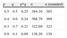
When we have no a priori values for the proportions to be estimated, we can use p- and q-values of 50%. This is the least favourable situation, in the sense that it yields a larger sample size, as can be seen in Table 1. It is always advisable to use prior pilot studies capable of giving us an idea of the proportion we wish to estimate, in order not to draw more sample than is actually needed.
In the case of estimating means, when the variance is not known but the mean has been established, we can take a standard deviation (square root of the variance) equivalent to at least half of the mean, for example: to estimate a mean of 14 referred to haemoglobin, we can take a deviation (variance) of 7 (49), whereby the sample size for an error of two units and a 95% confidence level would be 48 subjects.
Experimental studiesIn the case of experimental or observational studies, calculation is made of sample sizes when comparing two proportions and two means.12 The size of the population N does not intervene in these calculations.
Comparison of two proportionsWhen considering the comparison of two proportions, for example the percentage improvement after the administration of two different antihistamines in patients with allergic rhinitis, the formula for calculating SS would be:
where n=number of patients required in each of the groups; p1=proportion in the usual treatment group; p2=proportion in the new treatment group; q1, q2=inverse of the above (q1=1−p1, q2=1−p2); p=mean value of the two proportions (p1+p2)/2; q=1−p; tα=value of the normal curve associated to type I error (α); the value of α is usually between 5 and 10%; tβ=value of the normal curve associated to type II error (β); the value of β is between 10 and 20%.Comparison of two meansThe formula for calculating SS when comparing two means would be as follows:
where n=number of patients required in each of the two groups; x1, x2=estimated means of the groups to be compared; s2=mean estimated variance of the two groups. If a pilot study has been made, this variance can be estimated as a weighted average of the variances of both groups:with s12, s22, n1, and n2 as the variances and initial sample sizes in each group, respectively; tα=value of the normal curve associated to type I error (α); the value of α is usually between 5 and 10%; tβ=value of the normal curve associated to type II error (β); the value of β is between 10 and 20%.Losses in sample calculationThe losses in a study are those subjects for which it has not been possible to obtain information, on the grounds that they were not available at the time of the investigation.12 Losses are due to different causes:
- •
Patients who abandon the study (for example, in a clinical trial);
- •
Individuals who do not wish to form part of the study (fail to answer a questionnaire, etc.);
- •
Individuals failing to report for the visit, revision, etc.;
- •
Subjects that cannot be located at the time of the study;
- •
Adverse effects with some of the treatments;
- •
Loss of information due to other reasons (measurement error, imprecision of the measuring devices, etc.).
In sum, the causes of loss can be grouped into three categories:
- •
Withdrawal or dropout;
- •
No participation of the subject;
- •
No location of the subject.
All these causes imply that the initially calculated sample size becomes smaller, thereby reducing the power of the study (for example, more often declaring that there are no differences between treatments when in fact there are such differences).
In order to avoid this restriction in sample size, once the latter has been calculated, we increase it by the expected or foreseeable percentage of losses, based on the following formula:
n′: definitive sample size; n: initial sample size; d: expected proportion of losses expressed as a fraction.The percentage of losses is estimated from pilot studies.
Example: in the study referred to calculation of the sample size for estimating the percentage of individuals with seasonal allergy in finite populations, a 2% loss rate is estimated in relation to the localisation of individuals participating in the investigation. On incrementing the initial size by this percentage of losses, we have:
With a total of 225 subjects we ensure that in the event of a 2% loss rate or lower, the precision will be as initially established (i.e., a margin of error of 5%) – the precision increasing (i.e., error decreasing) as the number of cases increases (fewer losses) and decreasing (increased error) as the losses increase.
Calculation of sample size with RThe calculations of sample sizes with the R program are made using software packages developed for specific purposes, such as epicalc,13 samplesize and pwr. In the present article we use epicalc, which must be downloaded and installed as a first step. The R packages can be accessed from http://cran.r-project.org/web/packages/, and the epicalc application is downloaded in compressed format suited for the corresponding operating system.
Once the package has been installed, it must be loaded every time we wish to use the program. The installation is carried out from the R menu, following the instruction Packages→Install package(s) from local zip files, and selecting the previously downloaded file in the corresponding folder. For loading the package we follow the instruction:
> library(epicalc)
or use the option Packages->Load packages, from the R menu.
We aim to calculate the SS for the same study proposed in the sections above (estimation of the prevalence of seasonal allergy).
The instruction used for both finite and infinite populations is:
where p=the proportion to be estimated; delta=accepted error (half of the confidence interval, with a default value of 5%); popsize=size of the population. In infinite populations this is left in blank (default value); deff=design of the effect, number of patients required for each sampled subject (default value 1); alpha=level of signification (default value 5%).Example:
Thus, 219 subjects are needed to estimate the prevalence of seasonal allergy in this population of 2000 individuals.
For infinite populations, the corresponding instruction would be:
In this case, 246 individuals are required.
Estimation of a meanEpicalc does not provide instructions for calculating the SS when we wish to estimate a mean in either finite or infinite populations. Instead, we create a function that serves for this purpose by simply entering the formula for the finite case (in the infinite case we enter a population size of over 100,000). The function will comprise the parameters needed to apply the formula: a t-value associated to the confidence level (generally 1.96), variance, the size of the population, and the accepted error.
On applying the function to the above described example of the estimation of the mean inspiratory reserve volume, we obtain the following:
We thus require 53 subjects in the case of a finite population, and 54 in the case of an infinite population.
Comparison of two meansThe instruction calculating the SS for comparing two means is:
where mu1: mean of the first group; mu2: mean of the second group; sd1: standard deviation of the first group; sd2: standard deviation of the second group; ratio: ratio of cases between the first and second group. The default value is 1 (i.e., the same sample size in both groups); alpha: level of significance. The default value is 5%; power: power of the test (1-beta). The default value is 80%.Example:
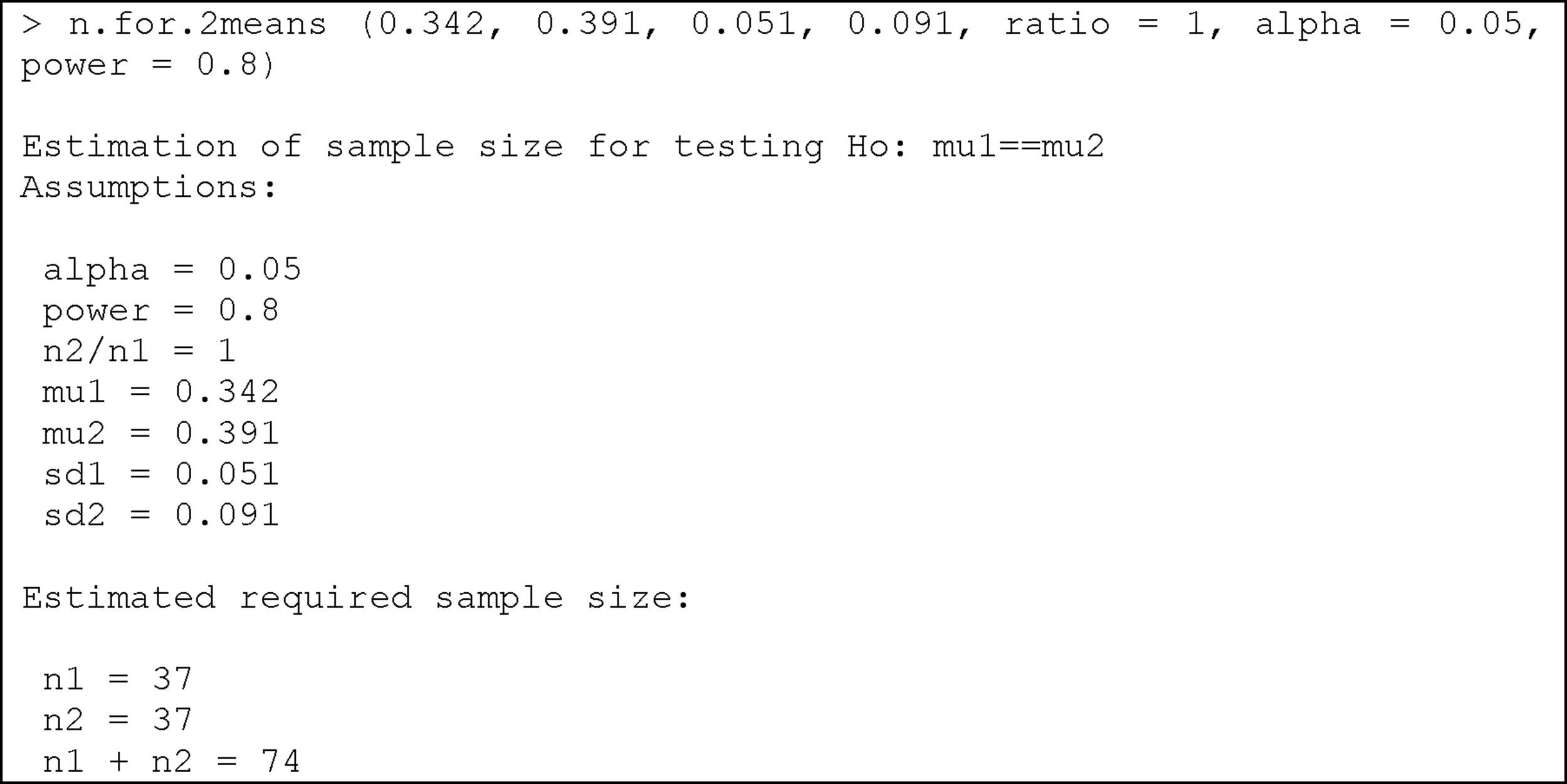
We wish to compare two egg white-free diets, with the purpose of lowering the specific IgE-KUi/l (immunoglobulin E) levels in individuals with egg white allergy. Previous studies have shown that the mean specific IgE level with diet 1 is 0.342, with a standard deviation of 0.051, while in the case of diet 2 the mean specific IgE level is 0.391, with a standard deviation of 0.091. We need to determine the sample size needed to evaluate differences between the mean specific IgE values after application of the two diets in two different groups of patients with egg white allergy, considering an alpha error of 5% and a beta error of 20%.
Substituting the values of the means, deviations, alpha and power of the test, we obtain:
We therefore need a total of 74 individuals with egg white allergy (37 per group) in order to detect differences in specific IgE between the two diets.
Comparison of two proportionsThe comparison of two proportions is performed in R with the instruction:
where in a way equivalent to the section above, the parameters to be entered are: p1: proportion of the first group; p2: proportion of the second group; alpha: level of significance. The default value is 5%; power: power of the test. The default value is 80%; ratio: ratio of cases between the two groups (by default we have the same number of cases in both groups).Example:
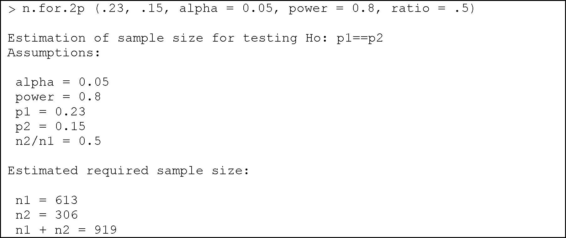
We wish to determine the percentage of dropouts following the administration of a treatment in two different groups of individuals. It is known that the dropout rate in group 1 can be 23%, versus about 15% in group 2. We need to determine the sample size required to evaluate whether there are differences in the percentages of dropouts between the two groups, knowing the frequency for group 2 to be half that of group 1, with an alpha error of 5% and a beta error of 80%.
Substituting in the formula, we have:
We thus need 613 subjects in group 1, and 306 in group 2.
It is estimated that there will be a loss rate of approximately 5% in each group, thus the above sample size would have to be expanded by this percentage:
We therefore would have to select 646 subjects in the first group, and 323 in the second.
The above operation can also be defined from the function:
Final considerationsIn this article we have addressed the calculation of sample size using the formulae defined to the effect, applied by means of the epicalc program to the type of studies most commonly found in health research. The instructions of this package refer to two-tailed hypotheses. In the case of a one-tailed hypothesis test, the formulae change, and these instructions are therefore not applicable.
The epicalc package comprises other instructions referred to the calculation of sample size for cases in which bioequivalence evaluations and non-inferiority tests are contemplated, and which are found in the documentation that comes with the package.
There are also other software packages14 for the calculation of sample size, such as pwr (calculation of power) or MBESS (for social and behavioural sciences), which are more complicated to use. In any case, we can always calculate any sample size in a study by simply applying the formula directly from the instructions line, or by defining a specific function as we have seen in some cases.


