

La escasez de información en el análisis de frecuencias de lluvias máximas diarias puede generar estimadores inefcaces para propósitos de diseño. Una forma de reducir estos errores es la aplicación de técnicas regionales, las cuales requieren que las estaciones involucradas pertenezcan a la misma región homogénea. En este trabajo se realiza una delimitación de regiones homogéneas de precipitación empleando un método multivariado basado en las técnicas de análisis de componentes principales y de agrupamiento jerárquico ascendente. La metodología propuesta se aplicó a una región del noroeste de México. Se concluyó que sólo se requieren los coefcientes de variación de los momentos-L y de la latitud, longitud y altitud de cada estación climatológica para definir las regiones homogéneas de precipitación, y que la inclusión o exclusión de información en las técnicas regionales tiene un impacto directo en la estimación de eventos asociados a diferentes periodos de retorno.
Lack of data in maximum daily rainfall frequency analysis can generate ineffcient estimates for design purposes. An approach to diminish these errors is to apply regional estimation techniques, which require that all stations be located at the same homogeneous region. In this paper, a delineation of homogeneous precipitation regions was made based on the multivariate methods of principal component analysis and hierarchical ascending clustering. A region in northwestern Mexico was selected to apply this methodology. It was concluded that only the coeffcients of variation of the L-moments, along with latitude, longitude and altitude at each climatological station are sufficient to define the homogeneous rainfall regions, and that either the inclusion or exclusion of information in the regional techniques has a direct impact on the estimation of events associated to different return periods.
The North American Monsoon System (NAMS) is defined as a pronounced increase in rainfall from an extremely dry June to a rainy July over large areas of the southwestern United States and northwestern Mexico (Adams and Comrie, 1997). The occurrence of NAMS is associated to atmospheric dynamics conditions and topographic characteristics, which interact with each other to cause a convective environment. This phenomenon can generate a high potential danger of flooding to residents in the country. In order to protect their lives and goods, it is very important to have a mathematical tool that may reduce the uncertainties in estimating design events for different return periods, which are needed in many hydraulic studies and projects such as food plain delineation or drainage works in cities.
In maximum daily rainfall frequency analysis, when information exists but not with the length of record required to provide accurate parameter estimates, the error of the estimated value for some return periods can be very large and inefficient for design purposes. A way of reducing this error is by applying a joint estimation model where information from nearby sites in the same region may be combined with the record of inadequate length. This approach will increase the amount of information and will provide a regional at-site estimate. An example of these regional models is the station-year technique, which is used to obtain a regional at-site estimate of the maximum daily rainfall for different return periods (Cunnane, 1988). These events are necessary to shape the intensity-duration-frequency curves (IDF) whose intensities i (mm/h) associated to certain duration d (h) and return period T (years) are used for designing hydraulic works.
The regional analysis correlates hydrological variables with the physiographical and climatological characteristics. Through these regional relations it is also possible to obtain flow estimates in rivers, as it can be seen in Wiltshire (1985), Stedinger (1983), Gingras and Adamowsky (1993), Burn (1988), Robinson (1997), Gutiérrez-López (1996), Escalante and Reyes (1998,2000), Pandey and Nguyen (1999), Ouarda et al. (2001), Gómez (2003), Skaugen and Vaeringstad (2005), and Ouarda et al. (2008).
The regional techniques require that the involved stations belong to the same homogeneous region. Since the inclusion or exclusion of information has a direct impact on the estimation of events associated to different return periods, adequately establishing that such homogeneity is achieved is an essential step to reduce the associated uncertainties.
A homogeneous region can be delineated by using geographical characteristics or statistical tests. Some works also have proposed indexes to evaluate the uncertainty and applicability of these methods: Nouh (1987), Cunnane (1988), Rosbjerg and Madsen (1995), GREHYS (1996a, b), Campos (1999), and Lin and Chen (2003).
In this work, the delineation of homogeneous regions is based on multivariate methods: principal component analysis (PCA) and hierarchical ascending clustering (HAC).
2Materials and methods2.1Principal component analysisPCA is a multivariate statistical technique highly descriptive, which is used to identify patterns on data in such a way as to highlight their similarities and differences. PCA can reduce the dimensionality of the data, transforming the set of r original variables or attributes in another set of s uncorrelated variables called principal components. The r variables are measured on each of the m sites. The order of the initial matrix of data is mr and it is restricted to m > r. After applying the PCA technique, the order of the resulting matrix is ms. This reduction of dimensionality is achieved with a little loss of information, which is considered non-significant to preserve the principal components.
PCA allows using either the correlation matrix or the covariance matrix. The first option gives the same importance to all and each of the variables. This can be convenient when the researcher considers that all the variables are equally relevant. The second option can be used when all the variables have the same units of measure.
The s new variables (principal components) are obtained as linear combinations of the r original variables. Components are arranged according to the percentage of variance that can be explained. In this sense, the first component will be the most important since it explains the largest percentage of the variance of data. Each researcher will decide how many components will be elected in the study.
PCA is performed in the space of the r variables and, in dual form, in the space of m sites. Variables and sites can be graphically represented by considering the first and second component as coordinate axes. A point-variable is represented by the coordinate corresponding to that variable in each of these components. The cloud of points-variables is located in a circular area of radius 1. The proximity between the point-variables indicates the degree of correlation between them. When the correlation is equal to one, the points coincide.
When the r variables are uncorrelated, r equally important components will be obtained. In contrast, when all variables have a perfect correlation, a simple component is generated. This component is a linear combination of the r equally weighted variables and explains 100% of the total variation.
The cloud of points-sites is not enclosed in a circle of radius 1. A point-site located at the extreme of one axis means that such station is closely related to the respective component. The opposite case indicates that the site has no relation with the two components. Proximity between sites is interpreted as similar behavior.
When there are several clouds of points that indicate the presence of a sub-population, and since the purpose of the study is to detect groups, the PCA achieves that aim.
2.2Hierarchical ascending clusteringHierarchical clustering is a method for grouping clusters, and seeks to build a hierarchy of these. There are two types of hierarchical clustering:
- a.
Agglomerative: This is an ascending approach where each observation starts in its own cluster, and pairs of clusters are merged as one moves up the hierarchy.
- b.
Dissociative: This is a descending approach where all observations start in one cluster, and splits are performed recursively as one moves down the hierarchy.
In order to decide which clusters should be combined (for the agglomerative approach), or where a cluster should be split (for the dissociative approach), a measure of dissimilarity between sets of observations is required. In most methods of hierarchical clustering, this is achieved by using an appropriate measure of distance between pairs of observations, in addition to a linkage criterion which specifies the dissimilarity of sets as a function of the pairwise distances of observations in them.
The choice of an appropriate metric will influence the shape of the clusters, as some elements may be close to one another according to a distance but farther away according to another distance. In this work the Euclidean distance will be the measure of distance between pairs.
If p = (p1, p2,..., ps) and (q1, q2,..., qs) are two points in Euclidean m-space with s-attributes (uncorrelated variables), the Euclidean distance from p to q is:

where p1 and q1 could be the average number of days with rainfall per year at sites p and q; p2 and q2 could be the average annual maximum of daily rainfall at sites p and q, and so on. In fact, Eq. (1) represents a distance among the different attributes of precipitation at two sites and not a physical distance between them.
The linkage criterion determines the distance between sets of observations as a function of the pairwise distances between observations. The linkage criteria used will be the Ward’s minimum variance method. Ward (1963) suggested a general agglomerative hierarchical clustering procedure, where the criterion for choosing the pair of clusters to merge at each step is based on the optimal value of an objective function. Ward’s criterion minimizes the total within-cluster variance. The pair of clusters with minimum cluster distance is merged at each step. To implement this method, the pair of clusters that leads to minimum increase in total within-cluster variance after merging is found at each step. This increase is a weighted squared distance between cluster centers. At the initial step, all clusters contain a single point. To apply a recursive algorithm under this objective function, the initial distance between individual objects must be proportional to the squared Euclidean distance.
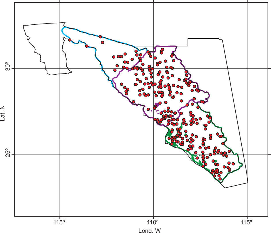
2.3Delineation of homogeneous regions2.3.1First scenario: Chaos simulationAll available variables are used without any prior consideration to build the site-variable matrix, and clusters are obtained based on HAC. In this first approach to grouping it is very common to observe that clusters present intersections among them.
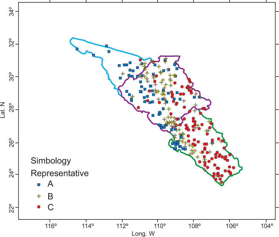
2.3.2Representative simulationA robust data matrix containing a set of variables with a high physical meaning by using HAC is formed. PCA is applied to obtain groups of variables associated with the four quadrants (principal components).
2.3.3Quadrants simulations (QS)In this stage, site-variable matrices are formed for each quadrant and HAC is applied to each of them.
2.3.4Fit and testing of sites clusters (F&T)PCA has to be applied to those variables whose quadrants presented the best spatial significance; then, groups containing the variables that explain 70 and 80% of the variance are gathered together. With these variables a new set of site-variable matrices is formed, which are analyzed with HAC.
2.3.5Final groupsThis step consists on the identification of optimal simulation based on scenarios and ratings from the previous phase. The procedure is applied by using:
- 1.
Some conventional moments of data (mean and standard deviation, among others).
- 2.
The L- coefficients of variation.
- 3.
The L-coefficients of variation plus the latitude, longitude and altitude at each climatological station.
L-moments are analogous to conventional moments but differ in that they are calculated using linear combinations of the ordered data (Hosking, 1990).
L-moments offer some advantages in comparison with conventional moments. As an example consider a dataset with a few data points and one outlying data value. If the ordinary standard deviation of this data set is taken it will be highly influenced by this point; however, if the L-scale is taken it will be far less sensitive to this data value. Consequently, L-moments are far more meaningful when dealing with outliers in data than conventional moments. Another advantage of L-moments over conventional moments is that their existence only requires the random variable to have a finite mean. Therefore, L-moments exist even if the higher conventional moments do not exist. L-moments are statistical quantiles derived from probability weighted moments. The first four L-moments are:


For a sorted sample x1, x2,..., xn in decreasing order, the values of the probability weighted moments β0, β1, β2 and β1 can be estimated by:

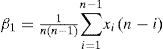
Additionally, a set of L-moments ratios or scaled L-moments can be defined by:
2.3.7Reliability of estimated quantiles


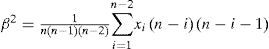
Once homogeneity is achieved and regions are defined, it is necessary to show whether or not the regional at-site estimate of the maximum daily rainfall for different return periods is more reliable than those computed using only a short sample (at-site estimate). This reliability can be quantified by several measures such as bias, root mean squared error and variance.
Let η be a quantile to be estimated; ωi, i= 1,...,ns the estimates obtained from each sample and ns the number of samples used in the experiment. Then, the bias and root mean squared error (RMSE) of the estimator ω may be computed as:
where m(ω) and S2(ω) are the mean and variance obtained from generated samples:
When estimating the parameters and quantiles of a distribution, it is convenient to have unbiased and minimum RMSE estimators. The RMSE involves both the variance of the estimator and the squared bias.
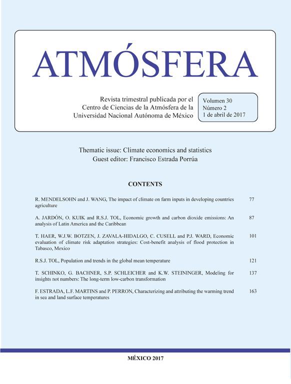
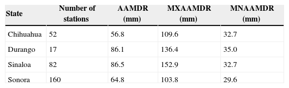
3Case studyA region located in northwestern Mexico, with a total of 311 climatological stations was selected to apply the proposed methodology (Fig. 1). Records of annual maxima for daily rainfall were gathered for the period 1965 to 2006 from the Rapid Extractor of Climatological Information version 3 (ERIC-III, by its initials in Spanish) database (IMTA, 2012). This period of time was selected because we had 88% of the available information. The inverse distance weighting (IDW) interpolation analysis was chosen for estimating missing data. The number of stations used and its average annual maximum of daily rainfall (AAMDR) by each Mexican state are presented in Table I (MXAAMDR and MNAAMDR stand for the maximum and minimum value of AAMDR, respectively).

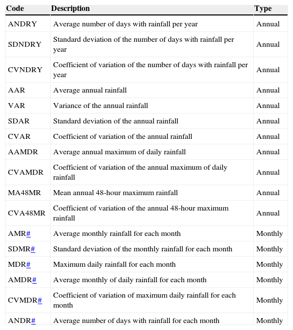
A first step to apply the PCA and HAC multivariate methods is the selection of variables to be analyzed. In order to achieve this, two sets of data were considered: The first one containing 11 annual variables and the second one consisting of 72 monthly variables, all of them from precipitation data (Table II). With this information a total of 83 variables were defined for each one of the 311 climatological stations. So, the first matrix of this analysis has 311 sites with 83 variables.
List of variables used in the delineation process.
| Code | Description | Type |
|---|---|---|
| ANDRY | Average number of days with rainfall per year | Annual |
| SDNDRY | Standard deviation of the number of days with rainfall per year | Annual |
| CVNDRY | Coefficient of variation of the number of days with rainfall per year | Annual |
| AAR | Average annual rainfall | Annual |
| VAR | Variance of the annual rainfall | Annual |
| SDAR | Standard deviation of the annual rainfall | Annual |
| CVAR | Coefficient of variation of the annual rainfall | Annual |
| AAMDR | Average annual maximum of daily rainfall | Annual |
| CVAMDR | Coefficient of variation of the annual maximum of daily rainfall | Annual |
| MA48MR | Mean annual 48-hour maximum rainfall | Annual |
| CVA48MR | Coefficient of variation of the annual 48-hour maximum rainfall | Annual |
| AMR# | Average monthly rainfall for each month | Monthly |
| SDMR# | Standard deviation of the monthly rainfall for each month | Monthly |
| MDR# | Maximum daily rainfall for each month | Monthly |
| AMDR# | Average monthly of daily rainfall for each month | Monthly |
| CVMDR# | Coefficient of variation of maximum daily rainfall for each month | Monthly |
| ANDR# | Average number of days with rainfall for each month | Monthly |
Using the 311 sites-83 variables matrix, clusters are obtained based on HAC. The behavior of the spatial distribution of the three groups of stations (A, B, and C) showed a high intersection among them (Fig. 2). These results led to the next stage of the study.
3.2Representative simulation.")
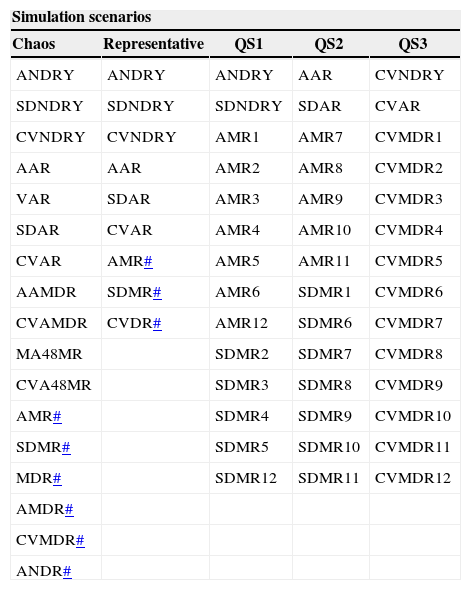
In this stage it is necessary to create a matrix containing a set of 42 variables with high physical meaning at 311 sites. The variables are presented in the column tagged as “Representative” (Table III).
List of variables used in each scenario of simulation.
| Simulation scenarios | ||||
|---|---|---|---|---|
| Chaos | Representative | QS1 | QS2 | QS3 |
| ANDRY | ANDRY | ANDRY | AAR | CVNDRY |
| SDNDRY | SDNDRY | SDNDRY | SDAR | CVAR |
| CVNDRY | CVNDRY | AMR1 | AMR7 | CVMDR1 |
| AAR | AAR | AMR2 | AMR8 | CVMDR2 |
| VAR | SDAR | AMR3 | AMR9 | CVMDR3 |
| SDAR | CVAR | AMR4 | AMR10 | CVMDR4 |
| CVAR | AMR# | AMR5 | AMR11 | CVMDR5 |
| AAMDR | SDMR# | AMR6 | SDMR1 | CVMDR6 |
| CVAMDR | CVDR# | AMR12 | SDMR6 | CVMDR7 |
| MA48MR | SDMR2 | SDMR7 | CVMDR8 | |
| CVA48MR | SDMR3 | SDMR8 | CVMDR9 | |
| AMR# | SDMR4 | SDMR9 | CVMDR10 | |
| SDMR# | SDMR5 | SDMR10 | CVMDR11 | |
| MDR# | SDMR12 | SDMR11 | CVMDR12 | |
| AMDR# | ||||
| CVMDR# | ||||
| ANDR# | ||||
Before the HAC analysis, a correlation analysis is applied to identify variables with a high degree of interdependence that could be eliminated. However, no variable was really inadequate, so this matrix was kept. The HAC analysis defined three regions that also presented intersections (Fig. 3). It was not possible to obtain a good independence among the three regions, so a new combination of variables was proposed.
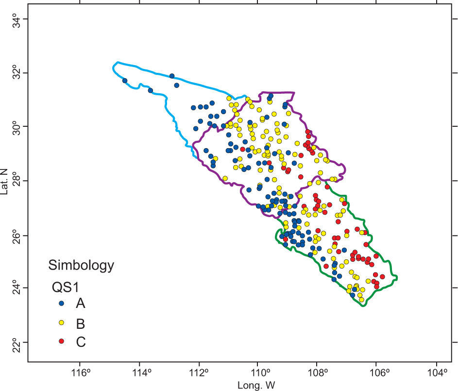
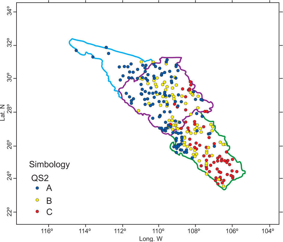
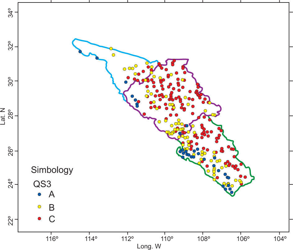
3.3Quadrants simulations: Scenarios QS1, QS2, and QS3.")
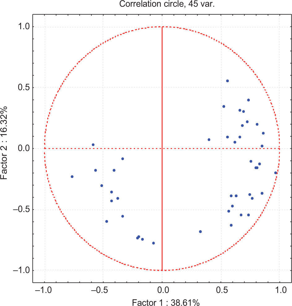
After PCA was applied to the 311 × 42 matrix, it was concluded that the first component explains 38.61 % of the population variance and the second one 16.32%. According to Figure 4, only a site-variable matrix could be constructed for the first, second, and third quadrant. It was not possible to construct the fourth quadrant because there was only one variable available. The variables created for dry season months fell into the first quadrant (QS1); the variables in the second quadrant (QS2) mostly correspond to rainy season months, and finally the third quadrant (QS3) comprises the coefficients of variation (Table III).

Once the site-variable matrices are constructed for each quadrant, the HAC procedure is applied for each of them. The resulting clusters are shown in Figures 5-7.


The groups obtained for the first (QS1) and second (QS2) quadrants do not have a defined pattern, because stations still continue to present some intersections among clusters (Figs. 5 and 6).
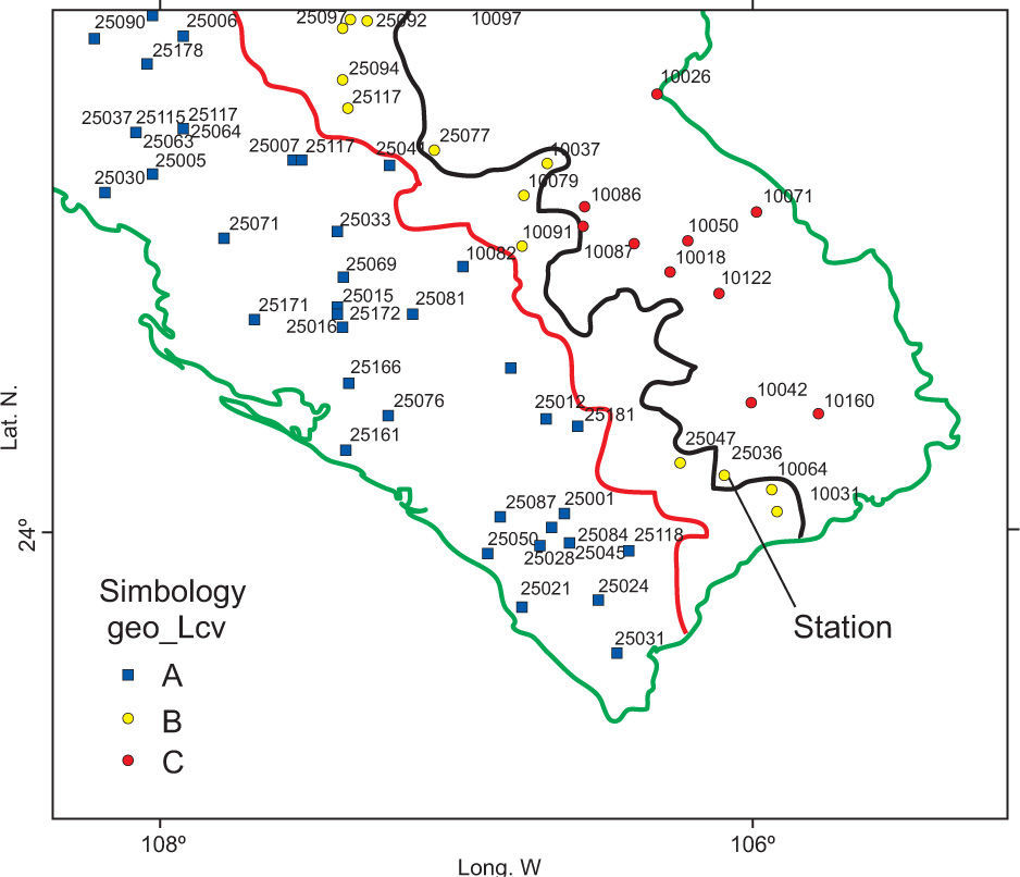
A better definition of clustering is achieved with a simulation process in the third quadrant (QS3). Intersections among groups significantly decreased (Fig. 7). Group A is located in the strip along the coast, with a short penetration inland and bounded by an imaginary line 40 km inland, meaning this is a coastal region. Group C corresponds to a mountain region; meanwhile group B is located in the central belt between groups A and C. These variables were considered for the last part of the study.
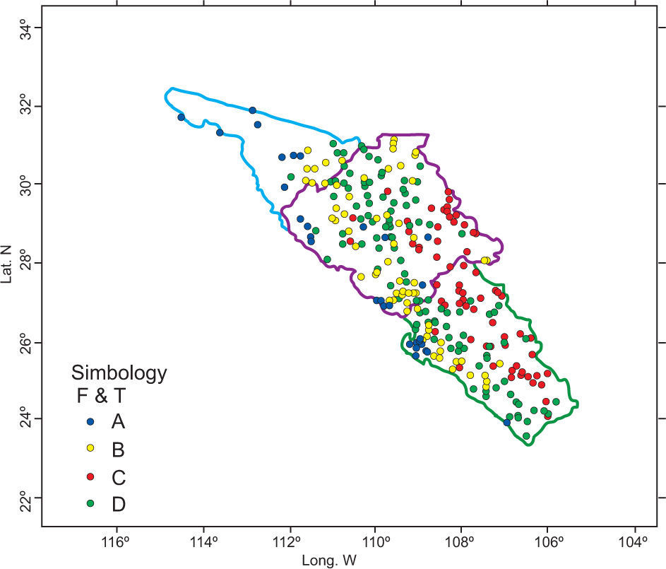
3.4Fit and testing of clusters of individuals (F&T)PCA was applied to variables from the third quadrant, which explained 70% of the variance. With this information a new site-variable matrix was created. This matrix is analyzed with HAC. Results (Fig. 8) show that groups A (coastal region) and C (mountain region) are stabilized; however, region B was divided into two parts (regions B and D).
3.5Final groups
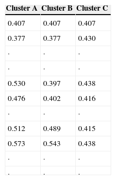
This phase of the study was conducted in order to achieve the optimization of homogeneous regions. Until this point, it was observed that the most important variables to define a homogeneous region were CVN-DRY, CVAR and CVMDR#. In order to improve the imulation process, these coefficients were substituted by the Z-coefficients of variation (L-cv) obtained by using Eq. (10). In this step some intersections among regions can be found (Fig. 9), however the formed clusters present a better definition than the F&T case.

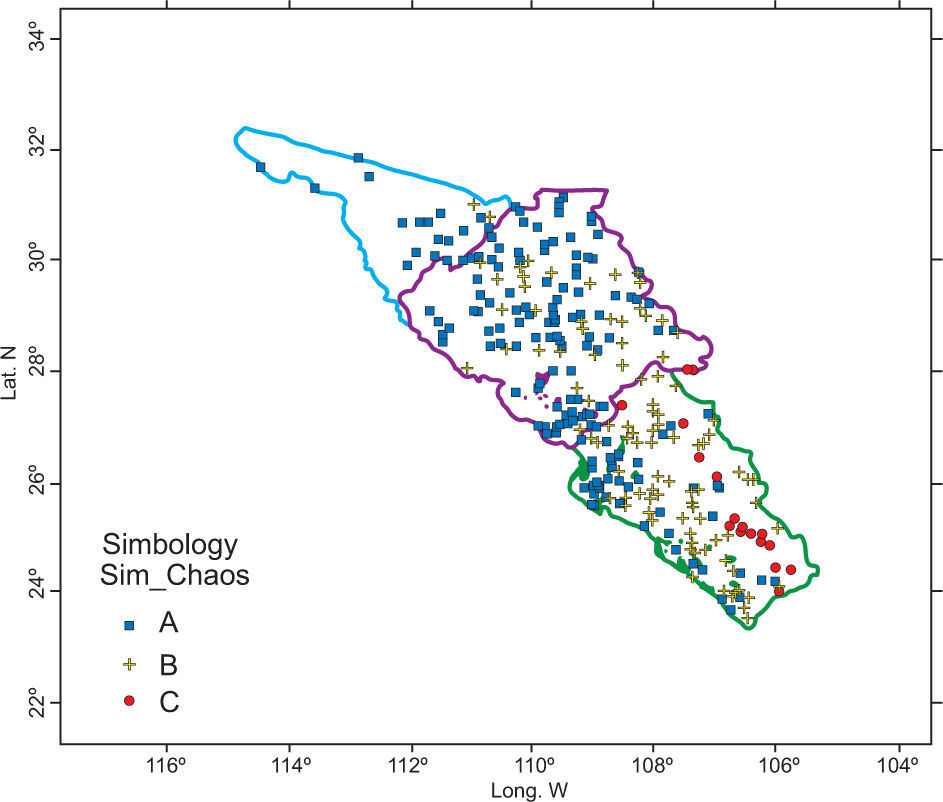
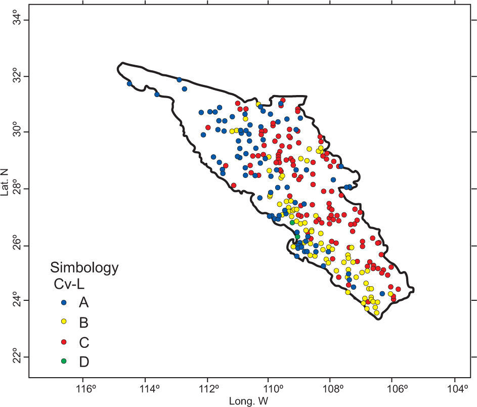
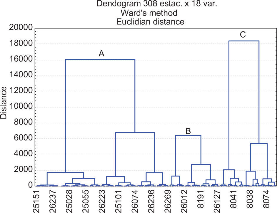
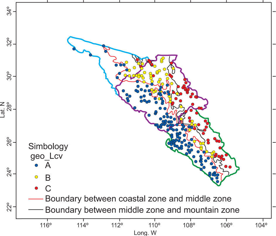
Finally, the geographical characteristics of latitude, longitude and altitude of each climatological station are added to the L-cv values from the former step. With this group of variables a new matrix is formed. The HAC analysis generated three well-defined clusters. A very important result was the migration of stations from the middle zone to the coastal region. So, group A would be located in the strip along the coast, bounded by an imaginary line 120 km inland. Group C corresponds to a mountain region; meanwhile, the middle zone was narrowed within both regions but extended along them. Figures 10 and 11 present the dendogram and clusters of the final simulation process.
3.6Comparison of k independent samples.")
.")
Some statistical tests can be used to show the independency of the chosen groups. For instance, Kruskal-Wallis test is used to find if k samples come from the same population or populations with identical properties as regards a position parameter. If M¡ (median) is the position parameter for sample i, the null H0 and alternative Ha hypotheses for the test are as follows:
H0: M1 = M2 = … = Mk
Ha: there is at least one pair (i, j) such that Mi ≠ Mj
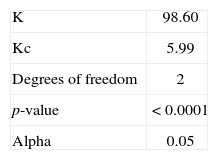
Calculation of the K statistic from the Krus-kal-Wallis test involves the rank of observations once the k samples or groups have been mixed. K is defined by:
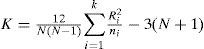
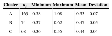
where ni is the size of sample i, N is the sum of ni variables, and Ri is the sum of the ranks for sample i. The distribution of the K statistic can be approximated by a chi-square distribution with (k-1) degrees of reedom. In this case, into each of the three groups only the average of the L-cv involved is considered to apply the Kruskal-Wallis test (Table IV). Results are presented in tables V and VI.
As K > Kc, then H0 is rejected and the three regions can be considered independent from each other.
3.7Comparison between at-site and regional at-site estimates of quantilesOnce homogeneity is achieved and regions are defined, it is necessary to show the effects of the inclusion or exclusion of information in the regional analysis. For this purpose, at-site and regional at-site estimates of the maximum daily rainfall for different return periods were obtained for the illustrative case of station number 25 036 (Fig. 12). For this station, the annual maxima of daily rainfall for the period from 1965 to 2006 were collected.

The reliability of these estimates was quantified by obtaining the RMSE values, following this procedure:
Case 1The at-site estimates of the maximum daily rainfall for return periods of 2-, 5-, 10-, 20-, 50- and 100-years are obtained by fitting the data to the normal (N), two-parameter lognormal (LN2). three-parameter lognormal (LN3), two-parameter gamma (GM2), three-parameter gamma (GM3), log-Pearson type 3 (LP3), Gumbel (G), and mixed Gumbel (MXG) distributions. The parameter estimation methods are moments (M), maximum likelihood (ML), L-moments (LM), maximum entropy (ME) and probability weighted moments (PWM). The best fit is selected according to the criterion of minimum standard error of fit (SEF), as defined by Kite (1988):

where gi, i = 1,..., n are the recorded events; hi, i = 1,..., n are the event magnitudes computed from the probability distribution at probabilities obtained from the sorted ranks of gi, i = 1,..., n; mp is the number of parameters estimated for the distribution, and n is the length of record.
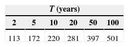
For this sample, the minimum value of SEF was obtained by fitting the MXG (ML) distribution. The maximum daily rainfall for each return period is presented in Table VII. These values are considered as the “true values” for long samples “η” in Eqs. (13) and (14).
Case 2The at-site estimates of the maximum daily rainfall for station number 25 036 are obtained by considering a set of 33 sub-samples of length n = 10 years (short samples). So, the record of annual maximum of daily rainfall for the periods 1965-1974, 1966-1975,…, and 1997-2006 are grouped. For each of them, at-site estimates of maximum daily rainfall are obtained by fitting the same distributions of the former case. These values are considered as the “estimated values” for short samples. The corresponding RMSE values are presented in Table VIII.
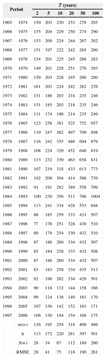
Maximum daily rainfall ω (mm) and RMSE for each of 33 sub-samples at station number 25 036 (case 2).
| Period | T (years) | ||||||
|---|---|---|---|---|---|---|---|
| 2 | 5 | 10 | 20 | 50 | 100 | ||
| 1965 | 1974 | 150 | 203 | 230 | 253 | 278 | 295 |
| 1966 | 1975 | 155 | 204 | 229 | 250 | 274 | 290 |
| 1967 | 1976 | 153 | 200 | 224 | 244 | 267 | 282 |
| 1968 | 1977 | 151 | 197 | 222 | 242 | 265 | 280 |
| 1969 | 1978 | 154 | 201 | 225 | 245 | 268 | 283 |
| 1970 | 1979 | 149 | 201 | 228 | 251 | 276 | 293 |
| 1971 | 1980 | 159 | 203 | 226 | 245 | 266 | 280 |
| 1972 | 1981 | 161 | 203 | 224 | 242 | 262 | 276 |
| 1973 | 1982 | 151 | 186 | 203 | 218 | 235 | 246 |
| 1974 | 1983 | 151 | 185 | 203 | 218 | 235 | 246 |
| 1975 | 1984 | 131 | 174 | 196 | 214 | 235 | 249 |
| 1976 | 1985 | 123 | 258 | 381 | 525 | 752 | 957 |
| 1977 | 1986 | 119 | 247 | 362 | 497 | 709 | 898 |
| 1978 | 1987 | 116 | 242 | 355 | 486 | 694 | 879 |
| 1979 | 1988 | 108 | 224 | 329 | 452 | 646 | 819 |
| 1980 | 1989 | 113 | 232 | 339 | 463 | 658 | 831 |
| 1981 | 1990 | 107 | 219 | 318 | 433 | 613 | 773 |
| 1982 | 1991 | 102 | 209 | 304 | 414 | 586 | 739 |
| 1983 | 1992 | 91 | 191 | 282 | 389 | 558 | 709 |
| 1984 | 1993 | 100 | 230 | 356 | 511 | 766 | 1004 |
| 1985 | 1994 | 113 | 241 | 334 | 428 | 553 | 648 |
| 1986 | 1995 | 86 | 185 | 259 | 333 | 431 | 507 |
| 1987 | 1996 | 77 | 176 | 251 | 328 | 430 | 510 |
| 1988 | 1997 | 80 | 179 | 254 | 330 | 432 | 510 |
| 1989 | 1998 | 87 | 186 | 260 | 334 | 432 | 507 |
| 1990 | 1999 | 85 | 184 | 258 | 333 | 432 | 508 |
| 1991 | 2000 | 87 | 186 | 260 | 334 | 432 | 507 |
| 1992 | 2001 | 83 | 183 | 258 | 334 | 435 | 513 |
| 1993 | 2002 | 92 | 190 | 262 | 334 | 429 | 501 |
| 1994 | 2003 | 90 | 118 | 132 | 144 | 158 | 166 |
| 1995 | 2004 | 99 | 124 | 138 | 149 | 161 | 170 |
| 1996 | 2005 | 107 | 130 | 142 | 152 | 163 | 171 |
| 1997 | 2006 | 106 | 130 | 144 | 154 | 166 | 175 |
| m(w) | 116 | 195 | 254 | 318 | 409 | 486 | |
| h | 113 | 172 | 220 | 281 | 397 | 501 | |
| S(w) | 28 | 34 | 67 | 112 | 189 | 260 | |
| RMSE | 28 | 41 | 75 | 118 | 190 | 261 | |
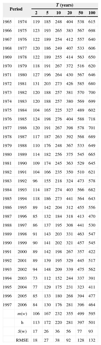
In the samples of case 2, differences among estimates “ω” can be considered very large. In order to improve them, it is possible to form a station-year record by adding information of stations belonging to the same homogeneous region. Again, as an illustrative case, only three neighboring stations are added to each of the 33 sub-samples of case 2. These stations are numbers 10 064, 10 081 and 25 047 (region B from Fig. 11). As already mentioned, each station has 42 years of available information (1965-2006), so the station-year records are formed by 136 values of annual maximum daily rainfall. These 33 station-year records are fitted to different distributions and regional at-site estimates of maximum daily rainfall are obtained. These values are considered as “regional estimates” for short samples with the inclusion of information coming from the same homogeneous region ω. The corresponding RMSE values are presented in Table IX.
Maximum daily rainfall ω (mm) and RMSE for each of the 33 station-year samples at station number 25 036 (case 3).
| Period | T (years) | ||||||
|---|---|---|---|---|---|---|---|
| 2 | 5 | 10 | 20 | 50 | 100 | ||
| 1965 | 1974 | 119 | 185 | 248 | 404 | 538 | 615 |
| 1966 | 1975 | 123 | 193 | 265 | 383 | 567 | 698 |
| 1967 | 1976 | 122 | 189 | 254 | 412 | 557 | 640 |
| 1968 | 1977 | 120 | 186 | 249 | 407 | 533 | 606 |
| 1969 | 1978 | 122 | 189 | 255 | 414 | 563 | 650 |
| 1970 | 1979 | 118 | 191 | 267 | 372 | 516 | 620 |
| 1971 | 1980 | 127 | 196 | 264 | 430 | 567 | 646 |
| 1972 | 1981 | 131 | 203 | 273 | 426 | 585 | 680 |
| 1973 | 1982 | 120 | 188 | 257 | 381 | 570 | 700 |
| 1974 | 1983 | 120 | 188 | 257 | 380 | 569 | 699 |
| 1975 | 1984 | 104 | 165 | 225 | 327 | 489 | 602 |
| 1976 | 1985 | 124 | 198 | 276 | 404 | 588 | 718 |
| 1977 | 1986 | 120 | 191 | 267 | 398 | 578 | 701 |
| 1978 | 1987 | 117 | 187 | 263 | 392 | 568 | 689 |
| 1979 | 1988 | 110 | 176 | 248 | 367 | 533 | 649 |
| 1980 | 1989 | 114 | 182 | 256 | 375 | 545 | 665 |
| 1981 | 1990 | 109 | 174 | 245 | 363 | 529 | 645 |
| 1982 | 1991 | 104 | 166 | 235 | 350 | 510 | 621 |
| 1983 | 1992 | 96 | 155 | 218 | 324 | 473 | 578 |
| 1984 | 1993 | 114 | 187 | 274 | 403 | 566 | 682 |
| 1985 | 1994 | 118 | 186 | 273 | 441 | 564 | 643 |
| 1986 | 1995 | 89 | 142 | 204 | 312 | 455 | 556 |
| 1987 | 1996 | 85 | 132 | 184 | 318 | 413 | 470 |
| 1988 | 1997 | 86 | 137 | 195 | 308 | 441 | 530 |
| 1989 | 1998 | 91 | 143 | 203 | 331 | 463 | 547 |
| 1990 | 1999 | 90 | 141 | 202 | 321 | 457 | 545 |
| 1991 | 2000 | 89 | 142 | 198 | 267 | 357 | 422 |
| 1992 | 2001 | 89 | 139 | 195 | 329 | 445 | 517 |
| 1993 | 2002 | 94 | 148 | 209 | 339 | 475 | 562 |
| 1994 | 2003 | 73 | 112 | 152 | 244 | 337 | 391 |
| 1995 | 2004 | 77 | 129 | 175 | 231 | 323 | 411 |
| 1996 | 2005 | 85 | 133 | 180 | 268 | 394 | 477 |
| 1997 | 2006 | 84 | 130 | 176 | 281 | 396 | 464 |
| m(w) | 106 | 167 | 232 | 355 | 499 | 595 | |
| h | 113 | 172 | 220 | 281 | 397 | 501 | |
| S(w) | 17 | 26 | 36 | 56 | 77 | 93 | |
| RMSE | 18 | 27 | 38 | 92 | 128 | 132 | |
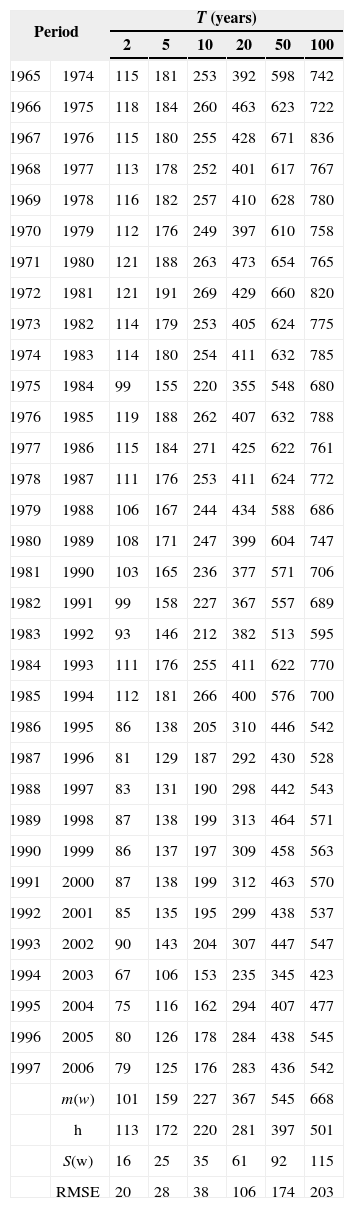
As it can be seen in Table VIII, a substantial gain is achieved by including some additional information to short samples. Additional information of stations 10 042 and 10 160 was added to each of the 33 station-year samples from case 3. These stations are located in a different homogeneous region (region C from Fig. 11). Each sample has a set of 220 values and after a frequency analysis the estimates of maximum daily rainfall were obtained. These values are considered as “regional estimates” for short samples with the inclusion of information coming from the same homogeneous region and from a different homogeneous region ω. The corresponding RMSE values are presented in Table X.
Maximum daily rainfall ω (mm) and RMSE for each of the 33 station-year samples at station number 25036 (case 4).
| Period | T (years) | ||||||
|---|---|---|---|---|---|---|---|
| 2 | 5 | 10 | 20 | 50 | 100 | ||
| 1965 | 1974 | 115 | 181 | 253 | 392 | 598 | 742 |
| 1966 | 1975 | 118 | 184 | 260 | 463 | 623 | 722 |
| 1967 | 1976 | 115 | 180 | 255 | 428 | 671 | 836 |
| 1968 | 1977 | 113 | 178 | 252 | 401 | 617 | 767 |
| 1969 | 1978 | 116 | 182 | 257 | 410 | 628 | 780 |
| 1970 | 1979 | 112 | 176 | 249 | 397 | 610 | 758 |
| 1971 | 1980 | 121 | 188 | 263 | 473 | 654 | 765 |
| 1972 | 1981 | 121 | 191 | 269 | 429 | 660 | 820 |
| 1973 | 1982 | 114 | 179 | 253 | 405 | 624 | 775 |
| 1974 | 1983 | 114 | 180 | 254 | 411 | 632 | 785 |
| 1975 | 1984 | 99 | 155 | 220 | 355 | 548 | 680 |
| 1976 | 1985 | 119 | 188 | 262 | 407 | 632 | 788 |
| 1977 | 1986 | 115 | 184 | 271 | 425 | 622 | 761 |
| 1978 | 1987 | 111 | 176 | 253 | 411 | 624 | 772 |
| 1979 | 1988 | 106 | 167 | 244 | 434 | 588 | 686 |
| 1980 | 1989 | 108 | 171 | 247 | 399 | 604 | 747 |
| 1981 | 1990 | 103 | 165 | 236 | 377 | 571 | 706 |
| 1982 | 1991 | 99 | 158 | 227 | 367 | 557 | 689 |
| 1983 | 1992 | 93 | 146 | 212 | 382 | 513 | 595 |
| 1984 | 1993 | 111 | 176 | 255 | 411 | 622 | 770 |
| 1985 | 1994 | 112 | 181 | 266 | 400 | 576 | 700 |
| 1986 | 1995 | 86 | 138 | 205 | 310 | 446 | 542 |
| 1987 | 1996 | 81 | 129 | 187 | 292 | 430 | 528 |
| 1988 | 1997 | 83 | 131 | 190 | 298 | 442 | 543 |
| 1989 | 1998 | 87 | 138 | 199 | 313 | 464 | 571 |
| 1990 | 1999 | 86 | 137 | 197 | 309 | 458 | 563 |
| 1991 | 2000 | 87 | 138 | 199 | 312 | 463 | 570 |
| 1992 | 2001 | 85 | 135 | 195 | 299 | 438 | 537 |
| 1993 | 2002 | 90 | 143 | 204 | 307 | 447 | 547 |
| 1994 | 2003 | 67 | 106 | 153 | 235 | 345 | 423 |
| 1995 | 2004 | 75 | 116 | 162 | 294 | 407 | 477 |
| 1996 | 2005 | 80 | 126 | 178 | 284 | 438 | 545 |
| 1997 | 2006 | 79 | 125 | 176 | 283 | 436 | 542 |
| m(w) | 101 | 159 | 227 | 367 | 545 | 668 | |
| h | 113 | 172 | 220 | 281 | 397 | 501 | |
| S(w) | 16 | 25 | 35 | 61 | 92 | 115 | |
| RMSE | 20 | 28 | 38 | 106 | 174 | 203 | |
Results indicate that there is a reduction in RMSE values when estimating the quantiles of a short sample (n = 10 years, case 2), taking into account the information from additional climatological stations oming from the same homogeneous region (case 3). However, when information belongs to different regions, RMSE values increase (case 4).
4ConclusionsThe delineation of homogeneous regions is based on multivariate methods: principal component analysis (PCA) and hierarchical ascending clustering (HAC)
A delineation procedure of rainfall homogeneous regions based on the multivariate methods of principal component analysis and hierarchical ascending clustering was presented. A region in northwestern Mexico was selected to apply this methodology.
The indiscriminate use of a large set of variables does not secure a robust result in cluster analysis. This study showed that the most important variables to define a rainfall homogeneous region were the coefficients of variation for series of number of days with rainfall per year, annual rainfall, and maximum daily rainfall for each month, which can be used as initial variables.
When coefficients of variation were substituted by their corresponding L-moments versions and the geographical characteristics were included into simulation, the HAC analysis allowed to obtain homogeneous regions that effectively preserve meteorological and orographic relationship (physical representation). So, three regions were settled, the first one from 0 to 500 masl, the second from 500 to 1500 masl, and the last one over 1500 masl.
The Kruskal-Wallis test was applied to prove that the chosen clusters are independent from each other, and they can be considered as different homogeneous regions.
Data-based results indicate that the inclusion or exclusion of information in the regional techniques has a direct impact on the estimation of maximum daily rainfall associated to different return periods. These differences could increase either the costs of hydraulic works or the risk of flooding, both of which affect people and their properties. Thus, it is very important to make a correct delineation of homogeneous regions.