


In this study, determination of heavy metal parameters and microbiological characterization of marine sediments obtained from two heavily polluted sites and one low-grade contaminated reference station at Jiaozhou Bay in China were carried out. The microbial communities found in the sampled marine sediments were studied using PCR-DGGE (denaturing gradient gel electrophoresis) fingerprinting profiles in combination with multivariate analysis. Clustering analysis of DGGE and matrix of heavy metals displayed similar occurrence patterns. On this basis, 17 samples were classified into two clusters depending on the presence or absence of the high level contamination. Moreover, the cluster of highly contaminated samples was further classified into two sub-groups based on the stations of their origin. These results showed that the composition of the bacterial community is strongly influenced by heavy metal variables present in the sediments found in the Jiaozhou Bay. This study also suggested that metagenomic techniques such as PCR-DGGE fingerprinting in combination with multivariate analysis is an efficient method to examine the effect of metal contamination on the bacterial community structure.
Pollution of coastal zones caused by heavy metals, such as Cd, Pb, Hg, and Ni, is one of the important environmental problems faced in many parts of the world.1 Heavy metal pollution can lead to severe changes in the composition of microbial communities that inhabit these zones.2,3 Microbial communities present in marine sediments primarily decompose organic matter derived from plant litter but also play a vital role in the transformation of pollutants.4,5 They can also influence the availability of heavy metals and are associated with other areas of the ecosystem.6,7 The influence of heavy metals on the decomposer subsystem and several other experimental systems has been studied in detail, such as, there are numbers of studies on the community structure of marine sediments from the continental shelf area is limited. Previous ecological and biological studies are mainly focused on the specific groups of bacterial communities that drive the biogeochemical cycling, e.g., ammonia-oxidizing bacteria.8–10 However, only a little is known on the dynamics of indigenous microbial populations that inhabit heavy metal contaminated coastal marine sediments. Although these studies provide vital information on the effects of heavy metals on bacteria found in marine sediments,11 they lack important ecological information, such as that offered by polymerase chain reaction (PCR) fingerprinting of the microbial community DNA extracted in these environments. It has been widely accepted that metagenomic techniques, such as PCR-DGGE (denaturing gradient gel electrophoresis) fingerprinting, are some of the widely used methods for examining the diversity of prokaryotic communities in environmental habitats.12–15 The PCR-DGGE profiles were used to construct a binary matrix for a quantitative comparison between different communities.16,17 These data were obtained either by visual scoring of gels or by commercially available software programs (for example, Bionumerics, Applied Maths, Belgium). These data can be presented as cluster analysis, e.g., an unweighted pair group method with arithmetic means,18 in which dendrograms are used to illustrate the relationship between different communities.19 Alternatively, PCR-DGGE profiles can be combined with multidimensional scaling, which is widely used to study the relationships between microbial diversity and various measured environmental parameters.20–22 Multivariate analysis has been utilized to determine the effect of metal contamination on bacterial community structure.23
Jiaozhou Bay is the largest semi-enclosed water body in the Yellow Sea (Fig. 1). It is located on the Chinese coast in the western Pacific Ocean. The environmental quality of this bay has deteriorated dramatically in the past three decades due to rapid increase in agriculture, industry, urbanization, and mariculture in the surrounding areas.24 This region contains very high levels of heavy metals in the sediments, due to the discharge of considerable amounts of heavy metals from the industrial plants located at the head of the Bay.25 The heavy metals levels in these regions were far exceed than their crustal average background values in the sediments at Jiaozhou Bay. The concentrations of the heavy metals in the sediments show a remarkable gradient ranging from high concentrations at the inner bay (Licunhe estuary and Haibohe estuary stations) to background levels at the outside of the bay (Shilaoren Beach station). The representative areas chosen for this study included the Lou Hill estuary, Licunhe estuary, Haibohe estuary, and Dagong Island that are located outside the area under study. The highest level of concentration of heavy metals was reported in Haibohe estuary wherein the concentrations of five heavy metals were 2.6–23.4 folds higher than their corresponding background values. In addition, the concentrations of Zn and Cu were much higher than that observed for other metals; the highest concentration of Zn was 1005.40×10−6, and that of Cu was 394.71×10⁻⁶. The concentrations of metals such as Zn, As, Pb, Cu, and Cd were higher than the corresponding background values in Licunhe estuary.26,27

The objectives of the present study were: (1) to use molecular techniques in combination with multivariate analysis to identify the sediment-associated microbial communities from both pristine and heavy metal-contaminated marine sediments in Jiaozhou Bay; (2) to assess the changes in the microbial community structure caused by heavy metal stress. In this study, the microbial communities inhabiting the Jiaozhou Bay were studied using PCR-DGGE fingerprinting profiles in combination with multivariate analysis. The concentrations of individual heavy metals present in the sediments were also determined.
Materials and methodsSite descriptionThe study location was Jiaozhou Bay, which is a semi-enclosed bay located on the south bank of the Shandong Peninsula, China. This bay is linked to the Yellow Sea by a very narrow entrance measuring only 3.1km across. It extends from 120°16′-120°17′E to 36°00′-36°02′N (Fig. 1). The average depth of this bay is 7m with a maximum of 64m. It covers an area of 362km2 of seawater and has a population of 7.2million. The long-term annual rainfall ranges from 340 to 1243mm with an average of 775.6mm, 58% of that in summer and 23% in winter. More than ten small seasonal streams empty into the bay with varying water and sediment loads, notably the Yanghe, Daguhe, Moshuihe, Baishahe, Haibohe, and Licunhe estuaries.27
Sample collection and environmental factor measurementsSediment samples were collected from two stations in Jiaozhou Bay and one station outside of the bay on December 30, 2011 using a 0.05m2 stainless steel box corer (Fig. 1). Seven samples were obtained from different points located at distances of 0.03, 0.06, 0.09, 0.12, 0.15, 0.18, and 0.21km from the Licunhe estuary, which has a waste input, and were numbered as LC1, LC2, LC3, LC4, LC5, LC6, and LC7, respectively. Similarly, five samples were obtained from different points located at a distance of 0.03, 0.06, 0.09, 0.12, and 0.15km from the Haibohe estuary, which has a waste input, and were numbered as HB0, HB1, HB2, HB3, and HB4, respectively. Another five samples were obtained from different points located at distances of 0.03, 0.06, 0.09, 0.12, and 0.15km from Shilaoren Beach and were treated as the low-grade contaminated control station and numbered as SLR1, SLR2, SLR3, SLR4, and SLR5, respectively.
The concentrations of heavy metals (V, Ni, U, Mo, Zn, Se, Sb, Co, Cr, Cd, Pb, As, Cu, and Hg) in the sediments were determined by graphite furnace atomic absorption spectrophotometry (GFAAS) using an AAnalyst 800 graphite furnace atomic absorption spectrometer (Perkin-Elmer, CT, USA).
DNA extraction and PCR-DGGE analysis of bacterial communitiesTotal community DNA was extracted with the BIO-101 DNA extraction kit (QBIOgene) from 0.5g of samples (wet weight). The sediment pellets were taken in lysis tubes containing a mixture of ceramic and silica particles, and DNA was extracted according to the manufacturer's protocol. The procedure combined highly energetic mechanical means (FastPrep Instrument, QBIOgene) in the presence of detergents and salts in the very first step to allow disruption of hard-to-lyse cells, minimize shearing of DNA, and inactivate nucleases. After DNA elution, a silica matrix was utilized to bind DNA, and the samples were washed with a salt/ethanol solution. The GENECLEAN Spin Kit (QBIOgene) was used as described by the manufacturer to re-purify the DNA. The yields of genomic DNA were determined after electrophoresis in 0.8% agarose gels stained with ethidium bromide under an UV transilluminator. The concentrations of DNA were estimated visually using the DL 15,000 DNA Marker (TaKaRa, China) in the agarose gels. The genomic DNA samples were diluted differentially to obtain concentrations of 1 to 5ng DNA to be used in the following step.28
Prior to DGGE analysis of the bacterial profiles, 16S rRNA gene fragments were amplified by PCR from total community DNA using the primer pair GC-F984 (5′-CGCCCGGGGCGCGCCCCGGGCGGGGCGGGGGCACGGGGGGAACGCGAAGAACCTTAC-3′)/R1378 (5′-CGGTGTGTACAAGGCCCGGGAACG-3′)29,30 using a DNA Engine (PTC-200) Peltier Thermal Cycler (Bio-Rad Laboratories, Inc). The reaction mixture was prepared as recommended by Costa et al.,28 with some modifications. Briefly, the reaction mixture (50μL) was composed of 1μL template DNA (1–5ng), 1x ExTaq buffer (TaKaRa, China), 0.2mM dNTPs, 3.75mM MgCl2, 4% (w/v) acetamide, 0.2mM of each primer, and 5U ExTaq DNA polymerase (TaKaRa, China). After a 5min denaturation step at 94°C, 30 cycles of 1min at 95°C, 1min at 53°C, and 2min at 72°C were carried out. A final extension step of 10min at 72°C was used to finish the reaction. Products were checked by electrophoresis in 1.5% agarose gels with ethidium bromide staining.
DGGE was performed with an INGENY phorU-2 system (INGENY International BV, Leiden, The Netherlands) using a double gradient gel containing 6–10% polyacrylamide (acrylamide/bisacrylamide, 37.5:1) with a gradient of 46.5–65% of denaturant (urea and formamide). The PCR products containing approximately equal amounts of DNA of similar sizes were separated on a gel containing a linear gradient of the denaturants. The run was performed in 1× Tris-acetate-EDTA buffer at 58°C at a constant voltage of 120V for 16hour. The DGGE gels were silver-stained according to Heuer et al. (2001).31
Statistical analysisThe denaturing gradient gels were scanned in the transmissive mode (Epson 1680 Pro, Seiko-Epson Corp. Suwa, Nagano, Japan) at high-resolution settings. The GELCompar® II v.4.0 software package (Applied Maths BVBA, Sint-Martens-Latem, Belgium) was used to analyze the community fingerprints of each denaturing gradient gel as recommended in the literature,32 with modified settings as described by Smalla et al. (2001).33 The comparison between samples loaded on different DGGE gels was performed using normalized values derived from known standards. The relative abundance of each phylotype (band) was estimated as the relative intensity of individual bands for each community (Lane) and was expressed as a proportion of the total community volume, thus normalizing the data and standardizing the loading differences. A binary matrix of identified bands was made for all gel lanes: the term ‘OTU’ is used to refer to each DGGE band. The Pearson correlation index for each pair of lanes was calculated as a measure of similarity between the community fingerprints. Cluster analysis was carried out by applying UPGMA (Unweighted Pair Group Method with Arithmetic Mean) to the matrix of similarities obtained. Then these data were subjected to canonical correspondence analysis (CCA) by using the software Canoco 4.5 for Windows (Microcomputer Power, Ithaca, NY, USA). Other data were analyzed according to previous literature.34,35 The concentrations of heavy metals in sediments were determined using the SAS general linear model (GLM) procedure (SAS Institute, Version 6, Cary, NC). The mean comparisons were carried out using ANOVA test and a least significant difference (LSD) test (p=0.05). Standard deviations, ANOVA results, and LSD results were recorded.
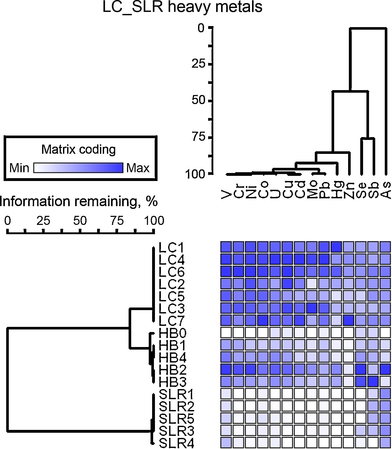
ResultsChemical analysis and similarity matrixThe concentrations of heavy metals in sediments are given in Table S1. A large variation in the concentrations of heavy metals in sediment samples was found. The concentrations of metals, such as Zn, As, Pb, Cu, and Cd, were higher in heavily contaminated Licunhe (LC) and medium contaminated Haibohe (HB) estuaries than those in the low-grade contaminated control station Shilaoren intertidal zone (SLR) (Fig. 2).
 occurrences in each sediment sample (rows). The number of blue boxes indicates that a given heavy metal has a high occurrence in that sediment sample. Dendrograms represent hierarchical clustering of sediment samples or heavy metals.")
The results of characterization of the metals obtained at the three sampling stations are shown in Table 1. The concentrations of all of the heavy metals investigated, with the exception of Sb and As, were significantly different between the different sampling stations (ANOVA, p<0.05). From the similarity matrix of the heavy metal parameters, very large differences in the sediment sample profiles were observed. The 17 samples obtained were classified into two clusters depending on the presence or absence of high contamination, and samples within the same sampling stations were generally clustered into a group (Fig. 2). The similarity matrices of the heavy metal parameters in LC and HB samples were significantly more related to each other. The cluster of highly contaminated samples was also divided into two sub-groups based on the stations from which they were obtained (LC and HB) and were characterized by 84% pattern similarity (Fig. 2). The greatest differences were observed between the two heavily contaminated stations (LC and HB) and the low-grade contaminated control station (SLR) (Fig. 2). DCA ordination of the heavy metals (data not shown) also showed that the samples could be classified into three groups on the basis of the station from which they were obtained.
Concentration of the heavy metals within each station.
| Heavy metals (ppm) | LC | HB | SLR | p | |||
|---|---|---|---|---|---|---|---|
| Mean | SD | Mean | SD | Mean | SD | ||
| V | 46.81 | 4.45 | 34.54 | 14.75 | 20.44 | 3.51 | 0.000 |
| U | 3.21 | 0.44 | 2.54 | 0.66 | 1.45 | 0.09 | 0.000 |
| Sb | 12.73 | 1.30 | 12.01 | 4.09 | 9.53 | 2.14 | NS |
| Cr | 57.73 | 9.61 | 37.70 | 20.13 | 10.26 | 2.00 | 0.000 |
| Co | 10.12 | 1.31 | 5.36 | 2.69 | 2.48 | 0.42 | 0.000 |
| Ni | 22.70 | 1.83 | 13.13 | 7.60 | 4.14 | 0.53 | 0.000 |
| Cu | 57.05 | 10.75 | 30.51 | 15.56 | 4.58 | 0.50 | 0.000 |
| Zn | 564.91 | 266.02 | 83.44 | 47.82 | 18.66 | 3.18 | 0.003 |
| Hg | 1.53 | 0.91 | 0.76 | 0.76 | 0.03 | 0.00 | 0.009 |
| As | 13.65 | 0.87 | 10.89 | 4.33 | 13.22 | 0.68 | NS |
| Se | 1.21 | 0.20 | 1.43 | 0.61 | 0.58 | 0.19 | 0.002 |
| Mo | 4.65 | 2.03 | 2.14 | 1.34 | 0.73 | 0.09 | 0.004 |
| Cd | 1.18 | 0.26 | 0.60 | 0.29 | 0.23 | 0.01 | 0.000 |
| Pb | 72.87 | 17.56 | 38.65 | 9.26 | 19.09 | 1.86 | 0.000 |
p, level of significance (ANOVA, p<0.05) between different stations (LC, n=7; HB, n=5; SLR, n=5); NS, not significant; LC, Licunhe estuary; HB, Haibohe estuary; SLR, Shilaoren Beach.
Some overlap occurred between DGGE bands observed in the heavily contaminated sediment samples (LC and HB) and the control sample (SLR). Around 100 defined DGGE operational taxonomic units (OTUs) were observed at a given site across the sample series. Approximately 54 of these OTUs were exclusively observed in the heavily contaminated sediment samples (LC and HB), and only 15 were found in the control samples (SLR). The remaining 31 OTUs were observed in both, heavily contaminated (LC and HB) and control (SLR) sediment samples. Two-dimensional hierarchical clustering of OTUs and samples, combined with a heat map of occurrence frequency, revealed groups of sample types and OTUs that had similar patterns of occurrence (Fig. 3). The distribution of OTUs among sample types was uneven; the majority of the observed OTUs were predominantly detected in either LC or HB sediment samples (groups B and C, Fig. 3). The OTUs in group A (Fig. 3) were most often found in SLR sediment environments.
 occurrences in each sediment sample (rows). The number of blue boxes indicates that a given DGGE band was observed in a larger proportion in that sediment sample. Dendrograms represent hierarchical clustering of sediment samples or DGGE bands.")
The comparison of profiles through the construction of similarity dendrograms revealed higher degree of similarity within one station than that between the samples from different stations. A fact that heavy metal contamination belongs to a specific grouping of microbial communities was preferred to visible (groups B and C, Fig. 3). UPGMA clustering of DGGE profiles revealed that the 17 samples were seemingly divided into two clusters depending on the presence or absence of high contamination. DGGE patterns in highly polluted samples were significantly more related to each other. The cluster of highly contaminated samples was also divided into two sub-groups based on their stations, which were characterized by approximately 25% pattern similarity (Fig. 3). CCA ordination of the same data also confirmed these groupings (Fig. 4). The samples from each station formed a cluster that was markedly different from others in both the analyses. These results showed that heavy metal variables in the sediments exert a strong influence on the community composition at the Jiaozhou Bay.
, HB (●), SLR (■). A group of samples in the same sampling stations is divided into the same enclosing envelope. The samples were divided into two groups (group A and group B) depending on the presence (HB, LC) or absence (SLR) of high contamination. The group B included the samples from low-grade contaminated control station (SLR). The group A of highly contaminated samples was divided into two sub-groups (group A1 and A2) based on their stations (HB and LC). Arrows indicate the direction of increasing values of the metal variable; the length of arrows indicates the degree of correlation of the variable with community data.")
CCA ordination of the OTU – environment relationships. Symbols: LC (○), HB (●), SLR (■). A group of samples in the same sampling stations is divided into the same enclosing envelope. The samples were divided into two groups (group A and group B) depending on the presence (HB, LC) or absence (SLR) of high contamination. The group B included the samples from low-grade contaminated control station (SLR). The group A of highly contaminated samples was divided into two sub-groups (group A1 and A2) based on their stations (HB and LC). Arrows indicate the direction of increasing values of the metal variable; the length of arrows indicates the degree of correlation of the variable with community data.
Twelve heavy metal variables were found to be significantly related (p<0.05) to bacterial composition in highly contaminated sediments. CCA ordination of DGGE patterns indicated that heavy metals affect the bacterial composition. The CCA explained 44.2% of the variation in the first two axes. Moreover, there were strong relationships between the OTUs and the heavy metal variables (OTUs and heavy metal correlations of the first two axes were 0.999 and 0.997, respectively).
In the CCA analyses, 50.7–71.6% of the cumulative variance of the OTUs – heavy metal relationship within each station was explained by the first two CCAs (Table 2). Heavy metal factors that correlated strongly with the genetic diversity of the bacterial communities differed among the stations. The strengths of the correlations between OTUs and heavy metal factors explained by the first two axes are shown in Table 2. The three strongest factors correlated with the axes (shown in bold) generally differed among the stations. The concentrations of Co, Zn, Hg, As, and Se were strongly correlated with one or both of the axes within each station. Additionally, the concentrations of As were strongly correlated with all sampling stations and played an important role (Table 2).
Weighted correlation matrix showing the relationships between OTU axes and environmental variables.
| Heavy metals (ppm) | LC | HB | SLR | |||
|---|---|---|---|---|---|---|
| Axis 1 | Axis 2 | Axis 1 | Axis 2 | Axis 1 | Axis 2 | |
| V | −0.1218 | −0.174 | 0.5192 | −0.464 | −0.6598 | 0.1421 |
| Cr | −0.0291 | −0.4455 | 0.3533 | −0.547 | −0.4957 | 0.2810 |
| Co | −0.0598 | 0.5549 | 0.6356 | −0.4342 | −0.3300 | 0.3183 |
| Ni | 0.1005 | −0.4973 | 0.4367 | −0.4536 | −0.2117 | 0.3611 |
| Cu | 0.0773 | −0.2347 | 0.4933 | −0.3405 | 0.0845 | 0.4293 |
| Zn | 0.0762 | 0.9036 | 0.2873 | −0.2502 | 0.2989 | 0.8420 |
| Hg | 0.7057 | −0.4008 | 0.1366 | −0.1411 | 0.7263 | −0.1899 |
| As | 0.5242 | 0.0560 | 0.1992 | −0.6720 | 0.8680 | 0.0094 |
| Se | 0.2599 | 0.1956 | 0.2976 | −0.0247 | 0.5057 | 0.8242 |
| Mo | −0.1019 | −0.2265 | 0.2932 | −0.4624 | 0.8483 | 0.3074 |
| Cd | −0.0784 | 0.4242 | 0.1914 | −0.4372 | 0.0050 | 0.5001 |
| Sb | −0.0635 | 0.3020 | 0.0283 | 0.6048 | −0.0301 | 0.2426 |
| Pb | 0.2412 | −0.0013 | 0.4615 | −0.4401 | 0.1233 | 0.5349 |
| U | 0.0022 | 0.0913 | 0.6078 | −0.2582 | −0.4108 | 0.6724 |
| Eigenvalues | 0.672 | 0.632 | 0.557 | 0.459 | 0.530 | 0.275 |
| Cumulative percentage variance of OUT-environment relation | 26.2 | 50.7 | 31.7 | 57.8 | 47.2 | 71.6 |
Heavily and medium contaminated stations: LC, Licunhe estuary; HB, Haibohe estuary; Low-grade contaminated control station: SLR, Shilaoren Beach. Bold type indicates the three strongest factors correlated with the first two CCA ordination axes.
DGGE bands are considered to be dominant unique sequence types (operational taxonomic units or OTUs) within the methodological constraints imposed by PCR.20,22 As reported earlier, two-dimensional hierarchical clustering based on both DGGE band relative intensities and sample chemistry results were used to determine whether microbial communities were related to environmental parameters.36,37 By combining with a heat map of occurrence frequency, the results revealed groups of samples from OTUs or heavy metal parameters that had both consensus matrices with similar patterns of occurrence. The majority of observed OTUs (groups B and C, Fig. 3) were predominantly detected in either of LC or HB sediment samples. The OTUs (group A) were most often found in the SLR sediment environment. This suggests that the dominant majority of OTUs (groups B and C) may be dispersed to be adapted to the contaminated sediment. The consistently dispersed bacterial taxa are strongly selected against heavy metals. Under the stress of combined heavy metal pollution, the shifts in bacterial community structures were significant between the polluted and the reference sediment samples. The increased OTUs in heavy metal polluted sediments could be caused by an acquired tolerance by adaptation, and a shift in species composition. The organisms that were already tolerant became more competitive and thus more numerous. We found that these results, similar to other investigators, further support the hypothesis that bacteria in heavy metal contaminated sediments are increased in number.38
Despite widespread use of DGGE profile data, a few of the studies have used these multivariate approaches to determine relationships between community composition and environmental variables as applied in this study. For example, a few studies identified the relationship between community composition and geochemical variables using PCA or CCA.10,39,40 The analysis, presented in this study, allowed the correlation of DGGE profiles with a wider range of environmental variables. A considerable number of studies have reported a strong relationship between community composition and environmental chemistry in marine sediments.10,39,41–45 Our results also suggest that community composition is strongly related to heavy metal variables in the sediments of Jiaozhou Bay. There were significant correlations between microbial community profiles and the concentrations of Co, Zn, Hg, As, and Se in the sediments. In the CCA analyses, 50.7–71.6% of the cumulative variance of the OTUs – heavy metal relationship within each station was explained by the first two CCAs (Table 2). Now, it appears reasonable to combine clustering analysis of DGGE banding patterns with ordination of the heavy metals using the CCA approach to analyze marine sediments. The bacterial community profiles in metal polluted sediment samples were dissimilar to those in the clean reference samples (Fig. 4). Similar results were also reported by Brad et al. (2008).46 Our results strongly support the hypothesis that environment controls the composition and distribution of microbial communities.47,48
In this study, molecular techniques in combination with multivariate analysis were used to identify the associated microbial communities in both pristine and heavy metals contaminated marine sediments in Jiaozhou Bay. However, it is important to bear in mind that a causal connection cannot be determined from statistical analysis alone. In addition, the obtained correlation values might be a result of other factors, as CCA disclosed only 44.2% of the variation on the first two axes; thus 55.8% of the variables remain unexplained. It must be noted, however, that DGGE has its own methodological limitations, and its fingerprinting patterns may not perfectly reflect the communities.49 The results of the DGGE and CCA analyses were intuitive, although the consequences may be oversimplified. Due to these shortcomings, inherent to all molecular techniques, the parameters calculated from the fingerprints must be interpreted as an indication and not an absolute measure of the degree of diversity in a bacterial community.50
As reviewed in literature, PCR-DGGE in combination with multivariate analysis is an efficient method for examining the effect of metals contamination on bacterial community structure.23 This was also confirmed by the observation that bacterial composition as depicted by DGGE was substantially related to heavy metals contamination. An in-depth study of the factors other than metals may explain the distribution observed. However, the information presented here might be useful in predicting the long-term effects of heavy metal contamination in the marine environment.
Conflicts of interestThe authors declare no conflicts of interest.
This work was supported by the program for National Natural Science Foundation of China (31471812, 31171809), and the Fundamental Research Funds for Jiangsu Academy of Agricultural Sciences (ZX(15)4007).