


Se tomaron en consideración distintos aspectos de algunas técnicas computacionales para el análisis AVOA (Amplitud Versus Offset y Azimut), para la composición de fracturas, en particular: utilizando amplitudes en lugar de coeficientes de refección, suavizando los datos sísmicos y el método de la estimación numérica para calcular la dirección. Se estimó un nuevo método de cálculo y se indica un nuevo método suavizado. Se compararan distintos métodos de cálculo en los datos sintéticos de superficie de reflección, con y sin ruido. Se obtuvieron propiedades de los métodos numéricos, dependientes de conjuntos distintos de los azimut y los offset. Se muestra una superioridad del nuevo método.
Different aspects of computational techniques for AVOA analysis (Amplitude Versus Offset and Azimuth) for fracture characterization are considered, in particular: using amplitudes instead of reflection coefficients, smoothing seismic data, and numerical methods for estimation of fracture directions. A new computational method and a new filter for smoothing are suggested. The different computational methods are compared in synthetic reflection surface data with noise, and without noise. Properties of the numerical methods in dependence on different sets of azimuths and offsets are obtained. It is shown a superiority of the new method.
The analysis of azimuthal variation in reflection coefficients, or AVOA analysis (Amplitude Versus Offset and Azimuth), is widely applied for detecting and mapping highly fractured zones with azimuthally-oriented vertical cracks (Mallik et al., 1998; Jenner, 2002; Sabinin & Chichinina, 2008). The AVOA techniques are based on the Rüger (1998) approximation for the reflection coefficients in HTI medium, and give principal symmetry directions of HTI medium.
Here, the computational aspects of AVOA techniques are considered, namely, applying amplitudes instead of reflection coefficients, smoothing the amplitudes, an incidence angle estimation, methods for obtaining the symmetry-axis angle, synthetic data for testing techniques, and a numerical experiment for investigating properties of the techniques. A new computational method for obtaining the symmetry-axis angle and a new filter for smoothing are suggested. All considered techniques are compared in synthetic anisotropic seismic data with noise, and without noise. The suggested new technique proved better than the others.
BackgroundThe methodology of AVOA analysis is based on the concept of azimuthal anisotropy caused for the most part by parallel vertical fractures. It leads to the azimuthal anisotropy of amplitudes, in particular, to azimuthal variation in reflection coefficients. Let a fractured reservoir be represented by a model of a transversely isotropic medium with horizontal symmetry axis (HTI medium). The PP-wave reflection coefficient R at the interface (or at the reflecting boundary) between weakly anisotropic HTI media (or between an isotropic medium and an anisotropic HTI medium) is defined by the approximate formula (Rüger, 1998):
where θ is the incidence angle, and ϕ is the source-receiver-line azimuth with respect to the coordinate axis x. The term A is the normal-incidence reflection coefficientwhere Z≡ρVP‖ is the vertical P-wave impedance, VP‖ is the vertical velocity (or velocity in the isotropy plane) of the P-wave, ρ i s density, Δ denotes the difference between the values of a parameter below and above the reflecting boundary, and the bar … indicates average of these values. VP‖=VP in the isotropic media.
The coefficient B(ϕ) is a so-called AVO gradient, which can be written (Rüger, 1998) as
where ϕ0 is the angle of the symmetry axis with the x−-axis. The term Biso is the AVO-gradient isotropic part (equal to the AVO gradient for isotropic media), and Bani is the anisotropic part of the AVO gradient.
The coefficient C(ϕ) can be written (Rüger, 1998) as,
where α≡ΔVP‖/2V¯P‖,β=12ΔεV, and γ=12ΔδV.
Above, Thomsen-style anisotropy parameters ε(V), and δ(V) are negative for HTI media, and they are equal to zero for isotropic media.
The main problem of AVOA analysis is to estimate the symmetry-axis angle ϕ0 from surface seismic data of amplitudes using numerical techniques.
The techniques of AVOA are based on equations (1) – (4). Note that equation (1) is intended for calculation of reflection coefficients, while in real data, one operates with amplitudes of reflected waves, not with reflection coefficients. This brings some problems which are discussed in the next section.
Using amplitudes instead of reflection coefficientsWhile the background of AVOA analysis is based on Rüger's equation for the reflection coefficient (1), in real data, AVOA analysis should use signal amplitudes. It is true that the amplitude is not equal to the reflection coefficient. Moreover, no picked instantaneous amplitude (sample) in the signal can be used instead of the reflection coefficient because the signal changes its form during propagation for many reasons. It seems that one should use an integral amplitude characteristic of the signal which adequately corresponds to the reflection coefficient. Let's call this characteristic simply by amplitude and denote it as P.
The estimated value of ϕ0 is very sensitive to the definition of P, especially for data with noise. I suggest the following procedure for definition of P which gives good and stable results. The procedure calculates an average value of a signal envelope in a time window. In calculating the envelope, the Fourier transform of this signal is used: F = F+ + F−, where F is spectrum, F+ is the part of spectrum corresponding to positive frequencies (ω≥0), and F− is the part of negative frequencies. The envelope of the signal is given by the absolute value of inverse Fourier transform of the spectrum with double F+, and F−≡0 (Sheriff & Geldart, 1983).
The sign of envelope is positive; therefore this approach is applicable only to seismograms with the constant sign of reflection coefficient in dependence on offset.
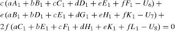
For data with noise, the envelope is noisy, too (see Figure 1). Therefore, smoothing is necessary.
 in time, and its envelope.")
For smoothing, an algorithm of discrete transformations of wavelet by filters is applied. Four symmetric filters are constructed for it: the low-pass (h0) end high-pass (h1) analysis filters, and the low-pass (h2) and high-pass (h3) synthesis filters. The right-hand part of h0 consists from the filter derived by Abdelnour & Selesnick (2004). The left-hand part of h0 is symmetric to it. That is
where a=M/32,M=2/2,b=4a, and n=8. The central value is c=1−M.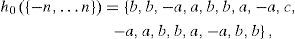
The high-pass analysis filter is constructed by formula h1(i) = (− 1)ih0 (n − i + 1) for i ≠ 0, and hl (0) = 0. The synthesis filters are calculated by formula h2(i) = (− 1)ih1 (i),h3 (i) = (− 1)ih0 (i), see (Abdelnour & Selesnick, 2005). The central values are h2 (0)=c and h3(0)=0.
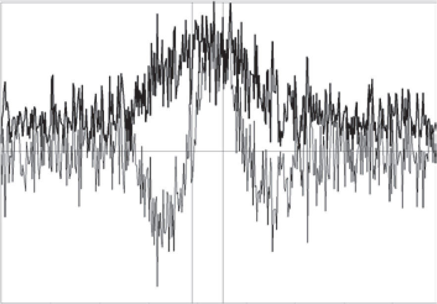
The smoothed signal is obtained by the decomposition algorithm; see Figure 2 (WSBP, 2012).

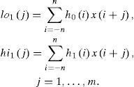
The input signal is x(j), j=1,…,m, m>>2n. It is decomposed into low and high components lo1(j) and hi1(j) in the first stage:
In the next stages (s=2,…, S), the each low component los-1(j) is decomposed by the same analysis filters.
After all stages of decomposition finishing, the stages of applying the synthesis filters are fulfilled in reverse order (s = S, S - 1,…,1):

The output signal y (j) is obtained finally:
where the fitting amplitude coefficient p can be approximately estimated by the formula p=1+0.057S, where S is the number of stages.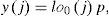
The advantage of this variant of discrete transformation algorithm in comparison with (WSBP, 2012) is the absence of shift functions in it due to applying the fully symmetric filters (i=-n,…,n).
It must be noted that the algorithm gives unsatisfactory results at the edges of the signal because of truncating the filters in 2n edge points. Therefore, it is necessary m>>2n.
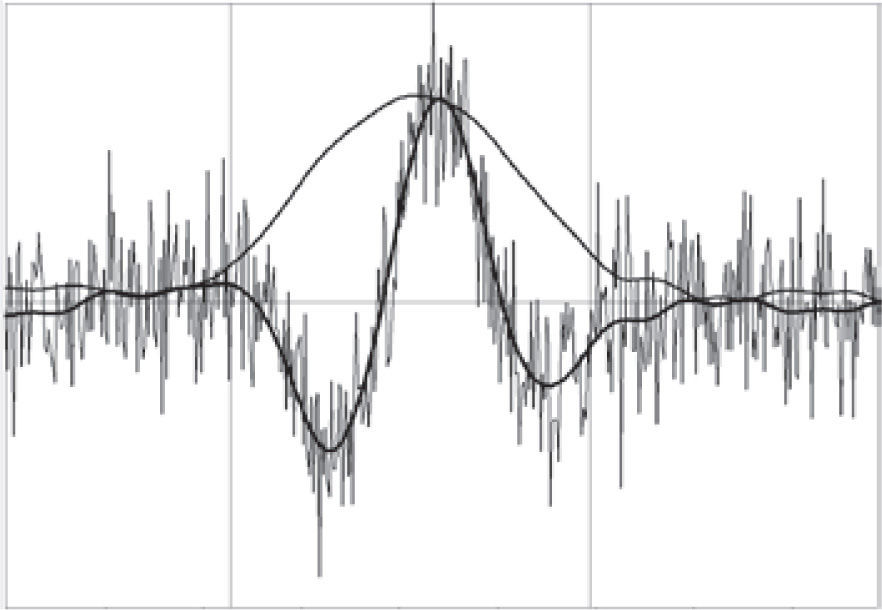
The result of smoothing the signal of Figure 1 by the 3-stage algorithm is presented in Figure 3. The smoothness of resulting curve increases with increasing S. Also with increasing S, the algorithm slightly deforms the resulting impulse in comparison with the parent impulse without noise. Optimum in the smoothness and in the conservation of form is observed at the value S=3.
, the smoothed signal (thick line), and the envelope of smoothed signal.")
The limits of time window for calculating P with the help of envelope can be chosen by different ways. I use the following way. From the envelope of signal e(t), the maximum em and nearest local minimums, left el and right er, are calculated. The left limit of the time window is set in the point where e = el + 0.15(em−el), and the right limit – where e = er + 0.15(em−el), see vertical lines in Figures 1, 3. Obviously, this algorithm correctly works only with smoothed signals.
Equation (1) should be rewritten for using the amplitudes. If the source and the receivers are at the earth surface, then the amplitude of reflected PP-wave can be expressed as
where cg is the coefficient of geometrical spreading (divergence) from source to reflection point for this wave, cg = cg (θ, ϕ), Pini is the amplitude of the source (the initial amplitude), and R is the reflection coefficient, R = R(θ, ϕ) in the equation (1).
The amplitude for the normal-incidence wave can be written as
where cg0 is the normal-incidence coefficient of geometrical spreading, which does not depend on (θ, ϕ), and A is the normal-incidence reflection coefficient, A = const, see equations (1) - (2). Then the reflection coefficient can be expressed as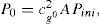

Therefore the equation (1) for the reflection coefficient R transforms into the following equation for the amplitude P:
where m=P0/A, and rg≡(cg0 / cg)2. This equation should be used in the AVOA techniques instead of (1).
Note that cg can be expressed as cg = c(θ, ϕ)/r in 3D space, where r is a half of travel path from source to receiver, and c depends on the direction of wave propagation (for isotropic media, c=const). In assuming a weak anisotropy, one may assume a weak dependence of geometrical spreading on incidence angle: c≈const for a given source-to-receiver line with azimuth ϕ. Then, for a homogeneous medium above the reflecting boundary,
where z is the normal-incidence ray path, and cg0 ≡ c / z. It is the approximate formula for divergent correction.
Also for multilayered media, the expressions for divergence correction can be found from Newman (1973). A practical methodology for the P-wave geometrical-spreading correction in layered azimuthally anisotropic media can be found from Xu & Tsvankin (2004).
The incidence angle estimationIn the case of n isotropic layers above the reflecting boundary, one can obtain the incidence angle θ = θn from a solution of the following non-linear equation for a:
where x0 is the half of offset, zi is the thickness of i-th layer, Vi is the velocity in i-th layer, and sin (θn)=aVn. For calculating the geometrical spreading, the travel path r=∑i=1nzi1−a2Vi2.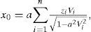
In the case of the reflecting boundary being the lower boundary of anisotropic layer, the problem is more complicated because the last layer is anisotropic, and the velocity Vn depends on θn in it and is not known beforehand.
The problem can be solved by Sabinin (2012). An advantage of his method is that the value Vn in the anisotropic layer is unnecessary for calculating angle θn and path r. However, it uses additionally the impulse from the upper boundary of anisotropic layer what complicates the technique. It gives results not sufficiently better than the method (8). Therefore, I use the simple method (8) here with setting an approximate value of Vn.
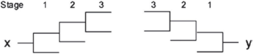
The methods for estimation of symmetry axis angle by AVOAUsually, 3D seismic data used in AVOA analysis are received from a system of receivers and sources spacing in nodes of a rectangle grid at the surface. The symmetry axis angle is calculated for a small square (for a bin) including a node of the grid, by using seismic traces which have the Common Middle Point (CMP) located in this bin. If such traces are few, then neighbor bins are combined into a superbin, and calculations are made for it. Therefore, a preliminary stage of the estimation is an extraction of seismic traces of the superbin from the seismic data for taking them into consideration.
For numerical methods of estimation of symmetry axis angle, one can use equation (6) as in Rüger's form:
as in the power form:where T* = rgP (θ, ϕ), T = (1−s)T*, s = sin2θ, t = cos2 (ϕ−ϕ0), a = P0, b* = mBiso, b = b*−a, c = mBani, d* = mα, d = d*−b*, e* = mΔδ(V)/2, e = e*−c, f=mΔε(V)/2−e* and m = P0/A.

The methods vary by simplifying ways applied, and can be separated into Sectored methods (S and SR), Linear methods (L and LR), and General method (G), where the letter ‘R’ denotes that the Ruger's form (9a) is used instead of (9b).
Sectored methodsThe method SR was suggested by Mallik et al. (1998) for the case of three azimuths with using equations (1), and (3). It took its perfect form in the work by Sabinin & Chichinina (2008) who used equations (6), (3), and (4). For this method, the traces of superbin are sorted by n azimuthal sectors. It is adopted that all traces of the sector have the same value of azimuth equal to the middle azimuth of the sector. Because of this, sectored methods introduce in ϕ0 an own error no more than a half of the sector size.
Here, the method S applied to equation (9b) is presented. If in the sector of azimuth ϕ (j=1, …, n), there are kj traces with incidence angles θj (i=1,…, kj) in the last layer above the target boundary, then one can write from (9b) for this sector j:
where Tij is the value T calculated from the trace i in the sector j. In each sector, Bj1=mjBj,Cj1=mjCj where mj=Pj/A, and Pj,Bj1,Cj1 are the fitting constants.
Having Tij and θi for all i in the sector j (kj≥3), one can calculate si=sin2θi, and then Pj, Bj1, and Cj1 from (10) by the least-squares method. For this, it is minimized the functional of error for each sector j:
For minimizing Fj, it is necessary to solve the system of three equations:

It gives: Cj1=b1f1−a1g1b12−a1c1,Bj1=f1−Cj1b1/a1, and Pj=u0BCj1−ABj1/kj, where a1=A2−Bkj,b1=AB−Ckj,c1=B2−Dkj,f1=Au0−u1kj,g1=Bu0−u2kj,

These calculations should be made for all sectors.
Then, the unknown value φ0 can be obtained from the system of equations of type (3), see (9b):
where j=1, …, n, and tj=cos2(φ−φ0). The unknown constants b1, and c1 have a sense: b1A=Biso−A, and c1A=Bani.
Equation (11) is transformed into more convenient form:
where Uj=Bj1/Pj, b0 = b1 + 0.5c1, c0 = 0.5c1, g = cos(2φ0), h = sin(2φ0), gj = cos(2φj) and hj = sin(2φj).
The system (12) has three unknowns (b0, c0, and φ0), therefore it should be n≥3 for obtaining solution. The system (12) has two solutions (two φ0 differing in π/2, and two c0 of opposite signs, correspondently), and is solved by the least-squares method, too. It is minimized the functional of error:
The following system of three equations should be solved:

It gives: tan2ϕ0≡hg=b1f1−a1f2b1f2−c1f1, c0=f1/(ga1+hb1), and b0=[u0−c0(Ag+Bh)]/n, where a1=A2−Cn, b1=AB−Dn, c1=B2−En, f1=Au0−u1n, f2=Bu0−u2n, A=∑j=1ngj,B=∑j=1nhj,C=∑j=1ngj2,
The condition for distinguishing symmetry-axis from fracture-strike directions is derived by Sabinin & Chichinina (2008), and uses equation (4). Here it is presented in more general form.
In terms of equations (9b), (10), and (11), equation (4) can be written as
where j = 1, …, n, d1 = (α − Biso)/A, e1 = (Δδ(V)/2 − Bani)/A, and f1=(Δε(V)−Δδ(V))/(2A).
When substituting the value φ0±π2 instead of φ0 into equation (14), the sign of the second term e1tj switches to the opposite sign, because equation (14) takes the form

The last term of equation (11)c1tj switches its sign, too. One can combine Δδ(V) = 2A(c1 + e1) from definitions to equations (11), (14), and conclude that the sign of Δδ(V) is switched, too. For calculating Δδ(V), it should be solved system (14) which is similar to (10) by the method of solution.
If the HTI layer is situated between isotropic layers then Δδ(V) must be negative for upper reflecting boundary of the HTI layer, and positive for lower boundary. If the calculated value of Δδ(V) has this sign then φ0 is the symmetry-axis angle. In opposite case, it is the fracture-strike direction.
It must be noted that Δε(V) = 2A(c1 + e1 + f1), and also can be used for distinguishing solutions because ε(V) and δ(V) have the same sign.
The formal condition that the second derivative of functional (13) must be positive in the minimum of functional can also be applied. Because of errors in data, it should be used as an additional condition to previous ones, and should have a form ∂2F/∂ϕ02> a small value.
Linear methodsThe method LR was suggested by Jenner (2002) for equation (1). It is not needed in sectoring data. All traces of superbin are taken into consideration together.
Here, it is applied to equation (9b), the method L. Equation (9b) is truncated after a line part respecting s. If the superbin has n traces(i=1, …, n), with incidence angles θi at the target boundary, and with azimuthal angles φi, then one can write the result of truncation in the form:
where Ti is the value T calculated from the trace i, si = sin2θi, b0 = b + 0.5c, c0 = 0.5c, g = cos(2φ0), h = sin(2φ0), gi = cos(2φi), and hi = sin(2φi).
The values si, gi, and hi are known because they can be calculated from headers of seismograms and parameters of medium. Let us consider the functional of error:
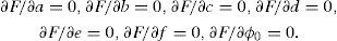
Functional F must be minimized over parameters a, b0, c0, and φ0. For this, it is necessary to solve the system of four equations:

Solution of system (17) gives the equation for obtaining φ0:
where A1=a1b1−a22,B1=a1c1−a32, A2 = a1b2 − a2a3, H1 = F2a1 − F1a2, and H2 = F3a1 − F1a3 in which a1 = nB − A2, b1 = nI − D2, c1 = nJ − E2, a2 = nG − AD, b2 = nK − ED, a3 = nH − AE, F1 = nf1 − Af0, F2 = nj2 − Df0, and F3 = nf3 − Ef0, and finally: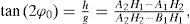
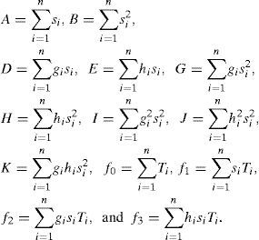
The other parameters are:
and a=(f0−b0A−c0gD−c0hE)/n.
From (18), one can see that the solution φ0 has a period of π2. This value of the period means that we must use an additional condition for understanding what value φ0 is the symmetry-axis azimuth. This condition may be Bani>0 if VS / VP>0.56 (Chichinina et al., 2003). In general case, it can be the condition ∂2F/∂ϕ02> a small positive value, where F is the functional of error (16).
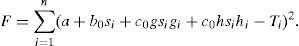
General method (G)The method is constructed by analogy with the GM method by Sabinin (2013). It is not needed in sectoring, too. All traces of superbin are taken into consideration together. If the superbin has n traces (i=1, …, n), with incidence angles θi at the target boundary, and with azimuthal angles φi, then equation (9b) can be written as:
where Ti is the value T calculated from the trace i, si=sin2θi, and ti=cos2(φi−φ0).
Let us consider the functional of error:

Functional F must be minimized over parameters a, b, c, d, e, f, and φ0. For this, it is necessary to solve the system of seven equations:
The six first equations of system (20) give a line system for deriving expressions for the parameters a, b, c, d, e, and f (for details, see Appendix).
The last equation of (20) can be transformed into a non-linear equation for obtaining φ0 (for details, see Appendix).
Thus, system (20) is non-linear on φ0, and is solved by the method of bisecting. It has more than one solution usually. From these local solutions, one chooses that one which gives a minimum for functional (19).
As was observed from calculations, the solutions of system (20) near the symmetry axis angle, and near the fracture strike angle give close values of functional (19). It means that additional criterions are practically needed for separating these directions. For the case of HTI layer situated between isotropic layers, it can be the condition of negative values for calculated ε(V) and δ(V) in the anisotropic layer, as above. For this, from definitions to equations (9b) and (2), one can calculate from the solution of (20) at the interface:
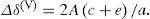
In the case of interface between anisotropic layers, it is needed additionally to know the predefined signs of Δε(V), and Δδ(V) for comparison.
The additional criterion can also be the maximum of second derivative of functional (19), ∂F/∂φ0.
Comparing the AVOA techniquesThe techniques using the methods above for estimation of symmetry axis angle were compared in ability to give the most precise value of φ0 for HTI medium. At present, reliable field methods of obtaining φ0 do not exist. Therefore, I generated synthetic seismograms for an artificial three-layer medium with the anisotropic layer in the middle by applying the technique by Sabinin (2012) of 2D wave modeling. I set φ0=60°, and derived models of the anisotropic layer for different values of φj by rotating the stiffness tensor for anisotropic layer (MacBeth, 1999) around z axis relatively to φ0. Anisotropic parameters en=0.35, and et=0.2 (see MacBeth, 1999) were used in the stiffness tensor.
Host rock velocity VP in three layers from above had the values 3200, 4000, and 4800 (the other variant was 3200), m/s, VS was twice less, densities were equal, and thicknesses of two first layers were 1600, and 400m. A source of explosion type generated one Ricker impulse of frequency 30Hz. Receivers were spaced over every 100m beginning from the source, and they measured z-component of velocity. There were 50 offsets, and 50 traces in each seismogram.
There were three goals: to investigate how the techniques behave on different sets of incidence angles, how the techniques are influenced by non-symmetry in φj relatively to φ0, and how the techniques are influenced by noise.
Therefore, for the first goal, I made calculations of φ0 for different intervals of offsets: from a minimum offset till a maximum offset, provided the minimum offset was fixed at the number one, and the number of maximum offset was changed from number 50 down to 3 in one set of the intervals; and the maximum offset was fixed at the 50-th, and the minimum offset was changed from number 1 to 48 in the other set of the intervals. Naturally, the maximum incidence angle θmax corresponding to the maximum offset, and the minimum incidence angle θmin corresponding to the minimum offset was also correspondently changed in these sets of offsets.
For the second goal, I obtained different sets of the synthetic seismograms corresponding to different azimuths, one seismogram for each azimuth. The sets of azimuths were uniform, and differed by symmetry. I did not aim to find the best or the worst set from them. I only supposed that a symmetric set can be better than an asymmetric one. I kept for testing the symmetric set of azimuths φj={−150°, −120°, −90°, −60°, −30°, 0°, 30°, 60°, 90°, 120°, 150°, 180°}, and the asymmetric set φj={85°, 95°, 105°, 115°, 125°, 135°, 145°, 155°, 165°}.
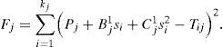
For the third goal, I took the best variant for the symmetric set of seismograms to eliminate the errors as due to the non-symmetry, as due to a finite-difference simulation when applying the artificial noise. The FD simulation by Sabinin (2012) uses PML boundary conditions which give non-visible (see Figure 4) but nonzero waves reflected from the boundaries of area. This slightly distorts the form of some synthetic impulses.

For the synthetic seismic data being quasireal, I added a random Gauss normal noise to the seismograms generated, different for each seismogram. Maximum amplitude of the noise was chosen as 10% of the maximum amplitude of the wave reflected from the top boundary of the anisotropic layer in the first trace of seismogram.
Finally, I added the noise to the seismograms of the asymmetric set.
All seismograms were smoothed by filters (5) in the techniques. High-frequency components of the noise are eliminated well after smoothing, as shown in Figure 3. It is principally impossible to eliminate low frequencies compared with the frequency of signal. Therefore, the signal after smoothing remains slightly deformed. I suppose that just these deformations affect the estimated value of φ0 in the case of noise.
The same sets of the time windows were used for all the techniques, and for all intervals of offsets.
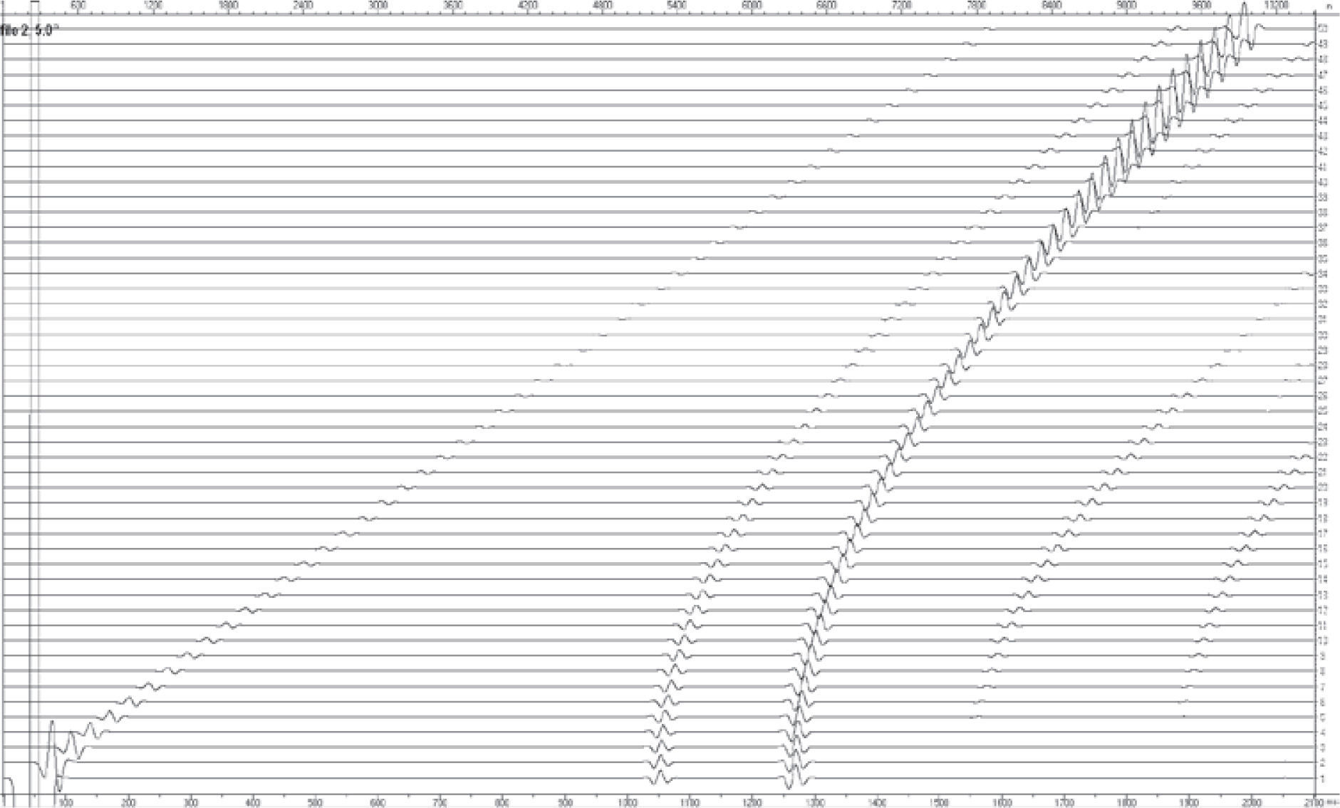
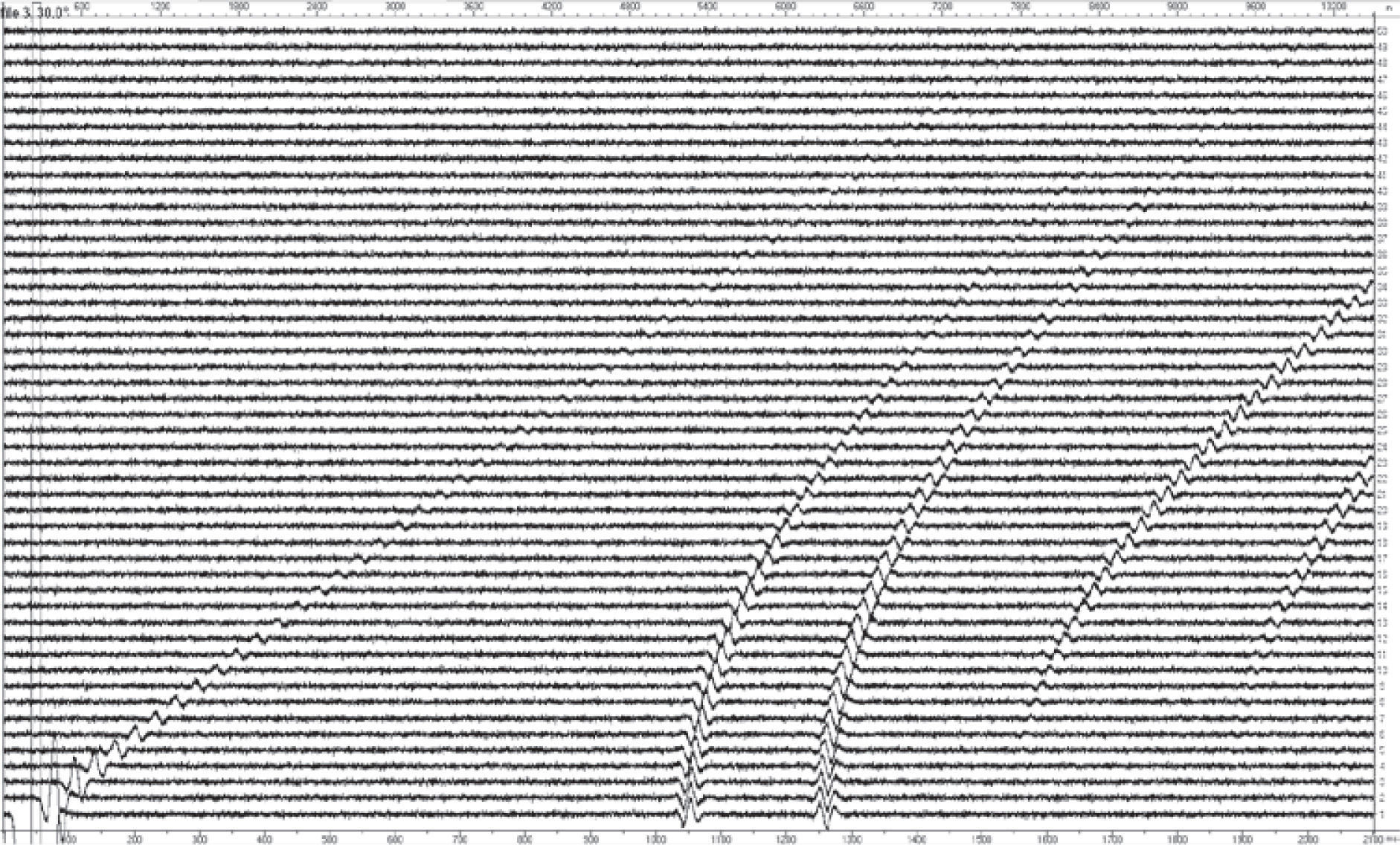
As illustration, in Figure 4, the seismogram without noise for azimuth 5° is presented for the variant of VP3=4800 m/s; and in Figure 5, the seismogram with noise for azimuth 30° is presented for the variant of VP3=3200 m/s.

As one can see from Figure 5, the amplitudes of noise reach really up to 50% of the maximum wave amplitudes in the middle traces, and up to 100% in the far traces.
The techniques were applied as to upper (1050 ms), as to down boundary (1250 ms) of the anisotropic layer.
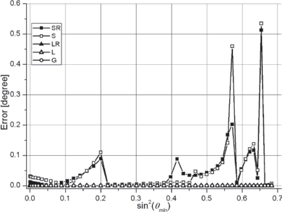
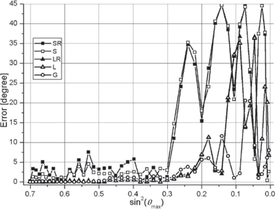
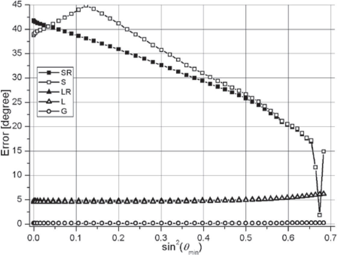
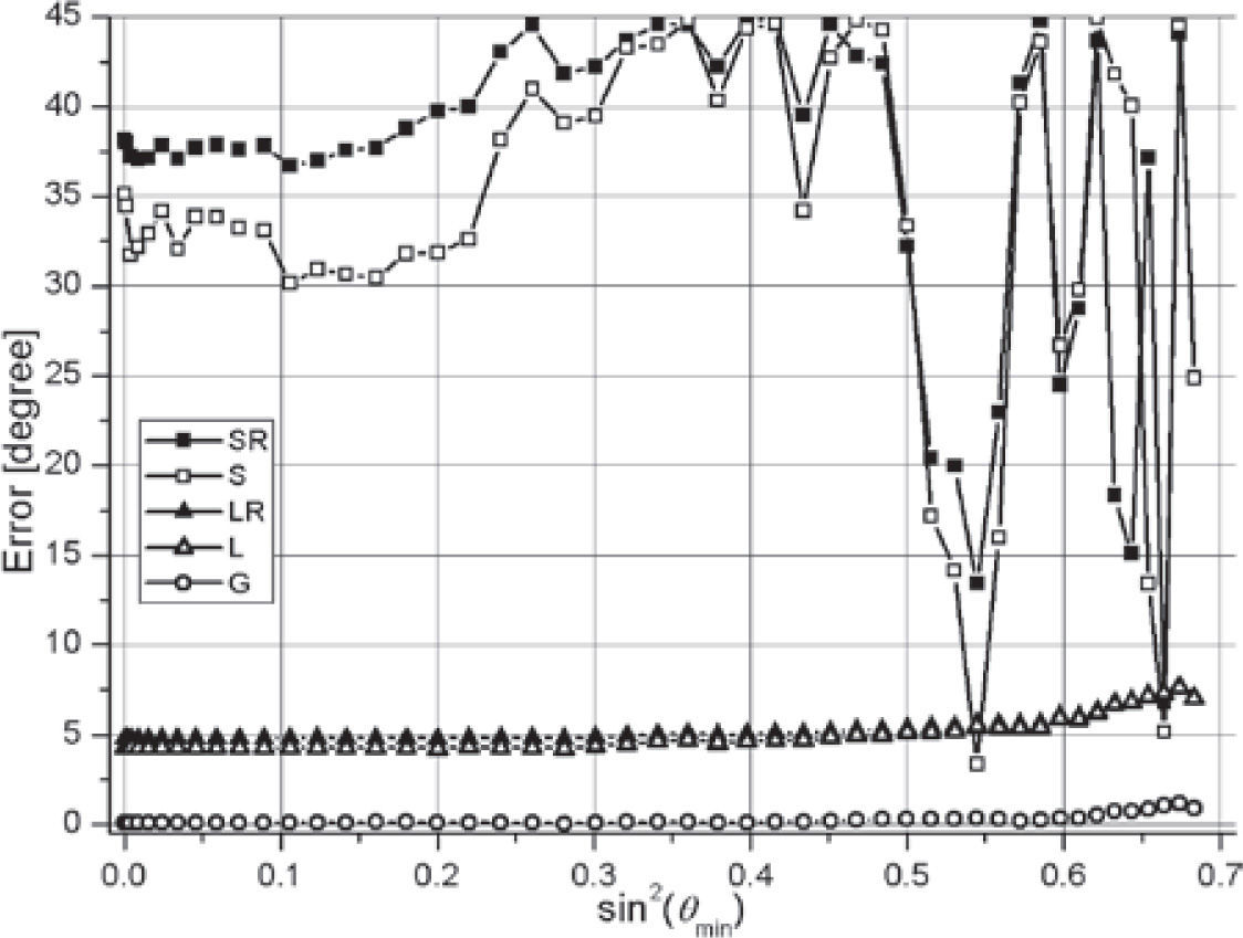
In Figures 6, 7, the error of estimated φ0 in degrees (difference with the correct value 60°) is presented for the symmetric set of azimuths and the upper boundary, variant VP3=3200. Figure 6 is for fixed θmin=0°, and Figure 7 is for fixed θmax=56.853°. The sectored methods show some instability for small values of θmax−θmin in comparison with the others. All methods increase the error in the case of small θmax (Figure 6).


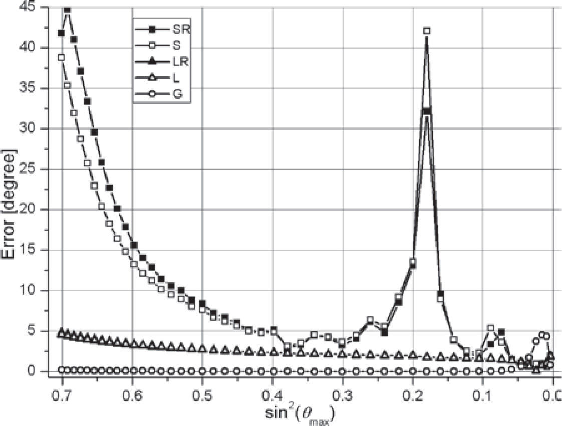
For the lower boundary and in the variant VP3=4800, the general and linear methods also show increasing errors for small θmax, and small θmax−θmin, see Figure 8, and Figure 9. However, the errors of these methods are sufficiently less than of the sectored methods.


In Figures 10, 11, the variant of Figs. 6, 7 with the added noise is presented. The sectored methods demonstrate so great errors and instability that can not be recommended for applying. The other methods show large errors only for small θmax (less than 30°).


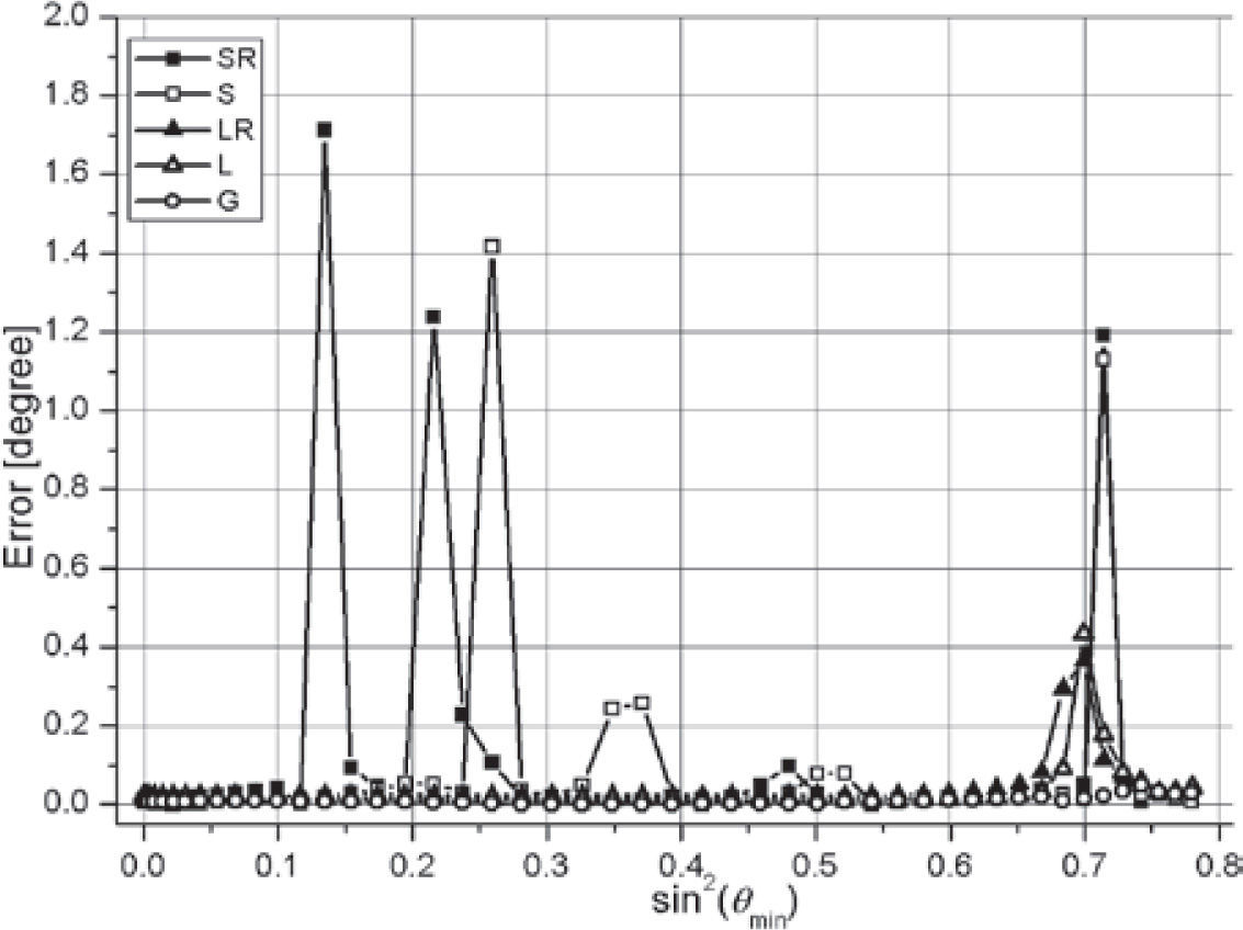
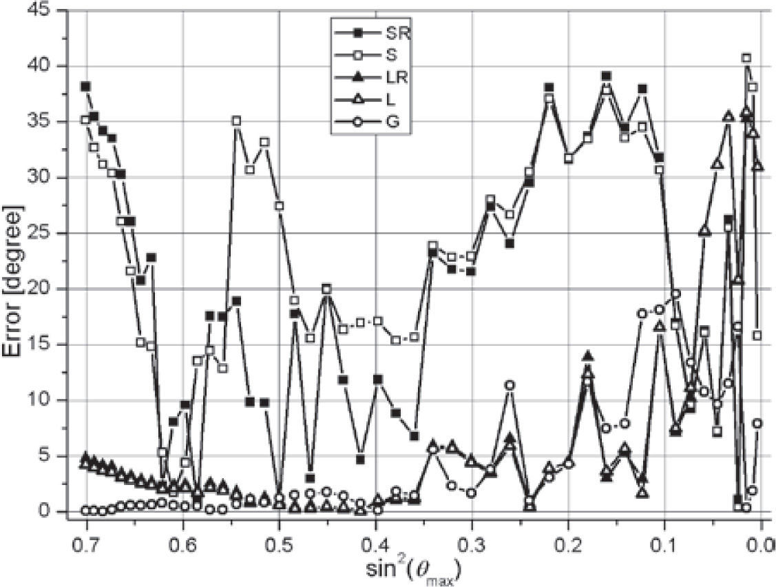
The asymmetric set of azimuths is presented by results in Figures 12–15. The variant of upper boundary and VP3=3200 without noise is presented in Figures 12, 13, and the same with the noise – in Figures 14, 15.


Typical peculiarities of the asymmetric set are: great errors of the sectored methods with instability in noised data, and stable large errors of the linear methods (up to 7°). The general method remains of small errors. The noise causes instability of all methods in the interval of θmax<36°, provided even the general method (G) gives large errors in this interval.
Discussion and conclusionSome unexpected results were obtained. The first is that the sectored S and SR methods are failed. They can be used only in seismic data without noise, and for mainly symmetric distributions of azimuths φ in the 3D data (Figures 6–9). This is too ideal conditions.
The second is that the linear L and LR methods have an additional nearly constant error in mainly asymmetric distributions of azimuths φ in the data (Figures 12–15). This error is probably connected with the truncation of high terms in equation (1) of Ruger, because the general method G has not such error. Therefore, the linear methods should be applied to azimuthally symmetric data.
The third is that the smoothing data with noise by simple filters (5) gives relatively stable estimated values of φ0 in a wide interval of incidence angles θ for the methods L, LR, and G (Figures 10, 11, 14, 15). The interval of instability is near the normal incidence, and has a width of θmax<40°, different in different variants (Figures 10, 14). For data without noise, this interval is θmax<10° (Figures 6, 8). Presence of the interval of instability is an intrinsic property of the formula (1) in connection with the least-squares method. Errors in amplitudes become relatively more with decreasing θ in definition of φ0 by equation (1).
The results show a superior of the general method (G). On the whole, its errors are less than of the others. Unfortunately, it has an intrinsic problem of choosing the right solution from the local solutions of non-linear system (20). All criterions described above do not guarantee the correct choosing. It is especially difficult in the interval of instability. All the methods have such problem of distinguishing solutions. The best in this sense is the method L. Its criterions are failed very rarely. Therefore, I recommend applying the method G in a coupling with the method L: after estimation of φ0 by L, the value φ0 is defined more precisely by G with expertly taking into consideration the local solutions of (20). The other recommendation is to avoid the interval of instability.
In applying to field data, the techniques can give worse results. The real data have much more interferences of waves than the synthetic data. It is practically impossible to clear each interfered wave of the other by filters. Distorted by this way impulses can lead to unpredictable results.
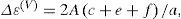
Let's define:
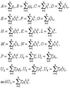
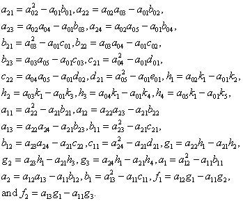
Then, from the first six equations of system (20), one can derive the formulas for unknown parameters:
where a01 = A2−Cn, a02 = AB−Dn, a02 = AC−Fn, a04 = AD−Gn, a05 = AE−Hn, b01 = B2−En, a02 = BC− Gn, b03 = BD−Hn, b04 = BE−Kn, c01 = C2−Ln, c02 = CD−Mn, c03 = CE−Nn, d01 = D2−Nn, d02 = DE−On, e01 = E2−Pn, k1 = AU0−U1n, k2 = BU0−U2n, k3 = CU0−U3n, k4 = DU0−U4n, k5 = EU0−U5n,
The seventh equation of system (20) takes a form:
where