En este trabajo se estima la sensibilidad de la temperatura del modelo WRF a cambios en la Radiación Solar Total (RST). Las simulaciones se realizaron para una región centrada en el Atlántico norte, incluyendo partes del Este de Norteamérica, Oeste de Europa y Noroeste de África. Para esto, se realizaron 4 simulaciones iguales, donde el único parámetro que se modificó fue la RST. Adicionalmente, se realizó una quinta simulación donde se cambiaron las condiciones iniciales atmosféricas, para comparar el efecto del cambio de la RST sobre la temperatura con el de un cambio en el día de inicio de la integración. Se compararon promedios mensuales de temperatura para cada simulación obteniéndose que tanto los cambios en las condiciones iniciales como los de la RST tienen un impacto medible en la temperatura de la región de estudio. Se presenta también una estimación de la sensibilidad del modelo usando parámetros adimensionales. Con estos experimentos numéricos encontramos algunos rasgos que permitirían distinguir entre los efectos de cambios de la RST y en las condiciones iniciales sobre la temperatura. Sin embargo, los cambios debidos al RST son de la misma magnitud que los cambios debidos a las variaciones en las condiciones iniciales. Se observa también que, en promedio y sobre toda la malla, la temperatura promedio no sufre cambios significativos ni ante cambios de la RST ni ante los de las condiciones iniciales.
The temperature sensitivity of the WRF model to changes in Total Solar Irradiance (TSI). The simulations were performed for a region centered over the North Atlantic Ocean, including portions of Eastern North America, Western Europe and Northwest Africa. Four simulations were run with different TSI values. Also, a fifth simulation was performed in which we varied the initial atmospheric conditions, in order to compare the effect on the temperature of both, changes in the TSI and initial atmospheric conditions. Comparing temperature monthly averages we found that changes in TSI and in the initial conditions have a measurable impact on temperature in the region of study. The sensitivity of the model using non-dimensional parameters was also estimated. The numerical experiments show some features that might allow to distinguish between the effects on the temperature due to changes in TSI from those caused by initial conditions. However, TSI changes are of the same order of magnitude than those of disturbances in the initial conditions. We also found that the mean monthly values of temperature over the full grid, did not present significant variations due to changes of either initial conditions or TSI.
Before the spatial era, it was believed that the solar radiation reaching the top of the atmosphere was constant with an approximate value of~1370W/m2. Since 1978, the radiometers on board of satellites have shown that the solar radiation is not constant, as it presents an increase of~0.1% between the minimum and the maximum of the 11-years solar activity cycle (Fröhlich, 2000). The Total Solar Irradiance (TSI) is the total electromagnetic power emitted by the Sun per unit area of cross section arriving at the mean Earth-Sun distance [Tiwari and Ramesh, 2007].
The TSI variations can affect the Earth´s climate through their direct influence on the mean global temperature or in some other indirect ways (e.g. Gray et al., 2010). General Circulation Models (GCM) estimate that a 2% increase of the TSI could produce an increase of~4°C in temperature. If we assume a linear scale, then 0.1% would produce a temperature increase of 0.2°C [CGER, 1994]. Comparing this temperature change with the temperature increase in the range of 1.5°C to 4.5°C estimated by the IPCC [2007], we could conclude that the temperature changes due to the 11- year TSI cycle change is small.
The stratospheric changes induced by the solar activity can influence the troposphere and the climate. Simulations using GCM suggest that solar UV changes modify the stratospheric ozone content and the temperature, affecting its latitudinal gradient. This modifies the stratospheric winds altering the tropospheric stability and impacting in several tropospheric dynamic processes including the intensity of the Hadley cell in low and subtropical latitudes and the low extra-tropical pressure systems. Although some GCM climatic simulations estimate a decrease of mean global temperature of 0.46°C for a 0.25% TSI reduction, some surface regions could cool and others could heat more than 1°C as a result of the advective changes produced by the differential heating of land and oceans [Haigh et al., 2005; Meehl et al., 2008; Barriopedro et al., 2008; Lee et al., 2008].
The aim of this paper is to estimate the sensitivity of the surface terrestrial temperature to changes in the TSI using the Weather Research and Forecasting Model (WFR). Although the WRF model can estimate other variables (Cipagauta et al., 2013), we choose the temperature as it is the most widely used climatic variable. We applied the model under several conditions: We use a regional model to observe the impact on México, although the boundary conditions constrain the behavior of the region, it allows us to use a higher resolution. The WRF model is applied only to the atmosphere, the sea surface temperature is prescribed. Finally, due to the computational cost required for each experiment the model was only ran for a single year.
The Weather Research and Forecasting Model (WRF)The WRF model is a next-generation mesoscale non-hydrostatic numerical weather prediction system designed to serve both operational forecasting and atmospheric research needs. Several institutions support the WRF project in order to achieve a better understanding of atmospheric processes and improved weather prediction [Skamarock et al., 2008]. In this study we used the WRF version 3.1.1 with the Advanced Research WRF (ARW) core. In all the simulations we applied Mercator projection and the schemes described in Skamarock et al. [2008] as follows:
- •
WRF Single-Moment 3-class for microphysics in a simple and efficient scheme that considers ice, snow and the Graupel processes, which are adequate for real mesoscale simulations.
- •
The Kain-Fritsch scheme for cumulus parameterization.
- •
The Yonsei University (YSU) scheme for the planetary boundary layer.
- •
The Rapid Radiative Transfer Model (RRTM) for the long-wave radiation.
- •
The Dudhia scheme for the short-wave radiation.
Four numerical simulations were run to investigate the impact of TSI on surface temperature. A fifth experiment was introduced to compare temperature sensitivity to changes in TSI and initial boundary conditions. We aim to estimate the variability of the temperature in each case. The simulation that corresponds to the base year represents the typical conditions of the region of interest. To study the sensitivity of the WRF model surface temperature due to TSI variations, we used non-dimensional parameters that estimate the surface temperature change as responses to radiation variations.
Description of Non-dimensional parameters techniqueTo relate TSI and temperature, we applied the radiative balance equation, widely used in atmospheric models. This relation is basically the Stephan-Boltzman expression for the black body radiation
where α the planetary albedo, S the solar radiation, σ is the Stephan-Boltzman constant, and T is the mean effective planetary temperature.
From equation (1), we calculated a non-dimensional parameter defined as
where k1 is a constant to be selected and T is the mean effective temperature. This parameter is a measure of the sensitivity of the corresponding variable [Szirtes, 2006].
In equation (2) the partial derivative is estimated by keeping as constants the other variables that could depend on T, and k1 is choose in such a way that βT is non-dimensional. Using equation (1) we find the partial derivative in (2), then we choose k1 as the inverse value of the partial derivative evaluated in a reference condition of radiation and temperature. Then the sensitivity parameter associated to temperature becomes:
where T is the model temperature for the radiative condition of our interest, T0 is the temperature of the base radiation. T and T0 can be daily or monthly averages, obtained from the model for different zones as well as over the full region of study, depending on the spatial and temporal behavior that we choose to examine
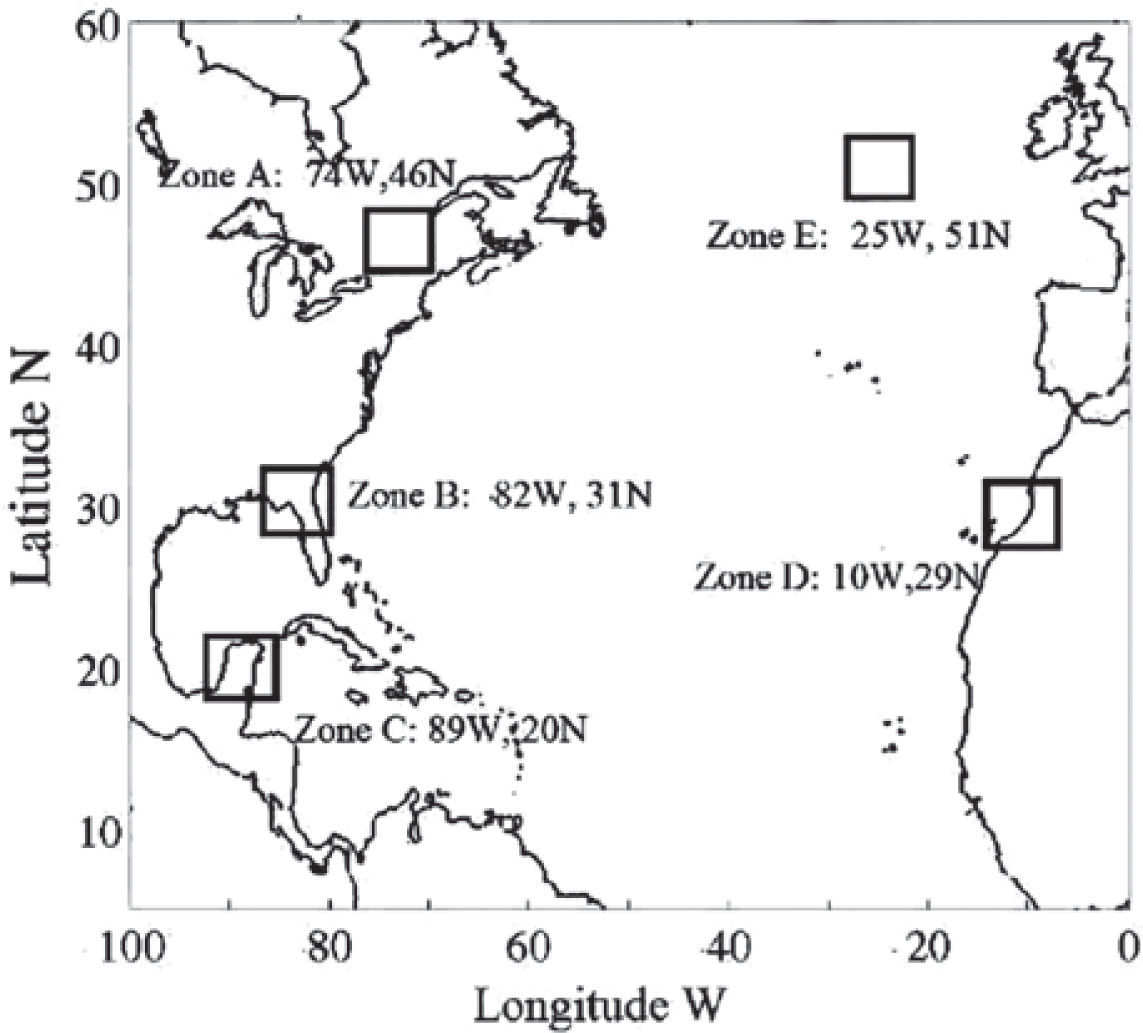
Simulation configurationWe choose a base year: September 1st of 1983 to August 31st of 1984. In this year the Sun was in the descending phase of its activity cycle showing intermediate activity, as it is approximately half way between the maximum and the minimum of solar activity. The simulation grid (see Figure 1) consists of a single domain centered over the North Atlantic Ocean between 0-100°W and 5-60°N, with a resolution of 30km, the region includes portions of Eastern North America, Western Europe and Northwest Africa. The initial and boundary conditions were taken from the NCEP/NCAR reanalysis project (Kalnay et al., 1996). We focus the analysis on five zones of the domain, where the surface temperature variations appear more noticeable. One exception was zone C, which was chosen due to the locations particular interest in this study.
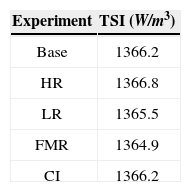
The intent of this study was to analyze temperature sensitivity to TSI variations using WRF model. Four simulations were run, each one with a fixed TSI value that vary among the simulations according to Table 1. The first simulation corresponds to the control experiment or base year, with a fixed TSI value similar to the one measured for the year 1983, which was a year half with a value between the maximum and the minimum of the 11-years solar cycle phase (http://www.pmodwrc.ch/php?topic=tsi/composite/SolarConstant). The measurements since the satellite era (1978) indicate that the TSI increase between the minimum and the maximum of the 11-years solar activity cycle~0.1%, this is mainly due to an interplay between superficial magnetic dark features such as sunspots and bright features such as faculae and network elements (Fröhlich, 2006). A higher solar activity year (HR) with a TSI increased by 0.05% corresponds to the second simulation. A year of lower solar activity (LR) with a TSI reduced by 0.05% corresponds to the third simulation. The fourth simulation was run with an estimate of the TSI for the next two solar activity cycles (Mendoza et al., 2010). This estimate indicates a period of lower solar activity and therefore lower solar irradiance. We named this numerical experiment as the future minimum radiation (FMR). Finally we performed a fifth simulation, using the control (base year) experiment but introducing the atmospheric conditions of the 2nd of September, 1983 as the initial conditions. We run this last simulation in order to compare the effects due to the TSI changes against the effects due to a variation of initial conditions.
We performed two different analyses with the surface temperature model results using monthly and daily averages. In the first analysis we calculated the monthly average differences between the HR, LR and FMR and the base year, those are D_HR for HR-Base, D_LR for LR-Base and finally D_FMR for FMR-Base, respectively. In the same way we indicate as D_IC the monthly average differences between the year with the changed initial conditions and the base year, that is D_IC=IC-Base. The second analysis is based on the calculation of the non-dimensional sensitivity parameter. We averaged the daily and monthly surface temperature means over the region of study. This average is used to calculate the sensitivity parameter through Equation (3), we take T_0 as the base year temperature over the whole domain and T is the model temperature over the whole domain.
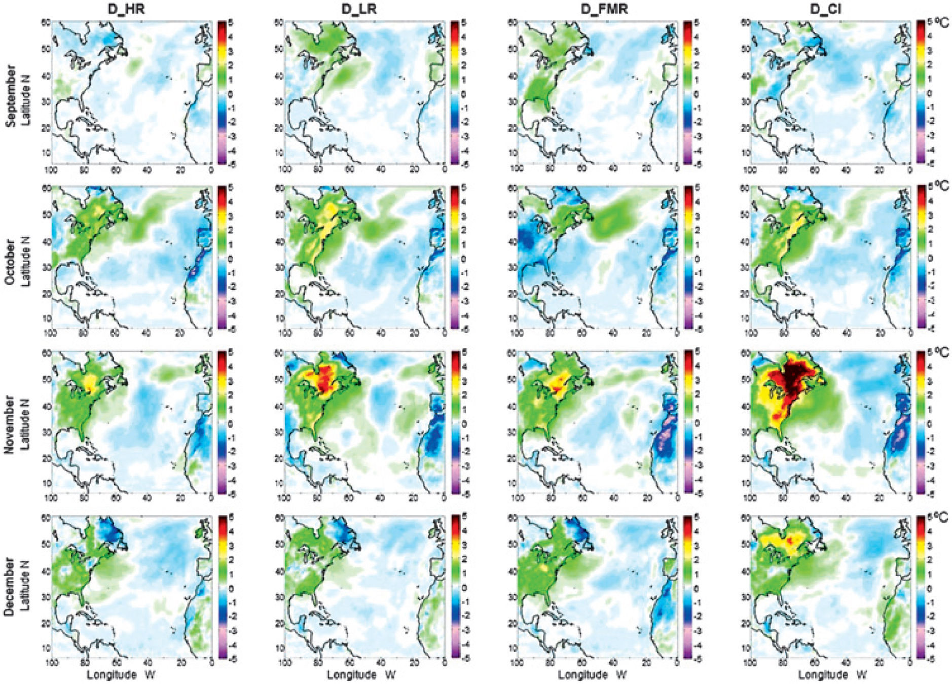
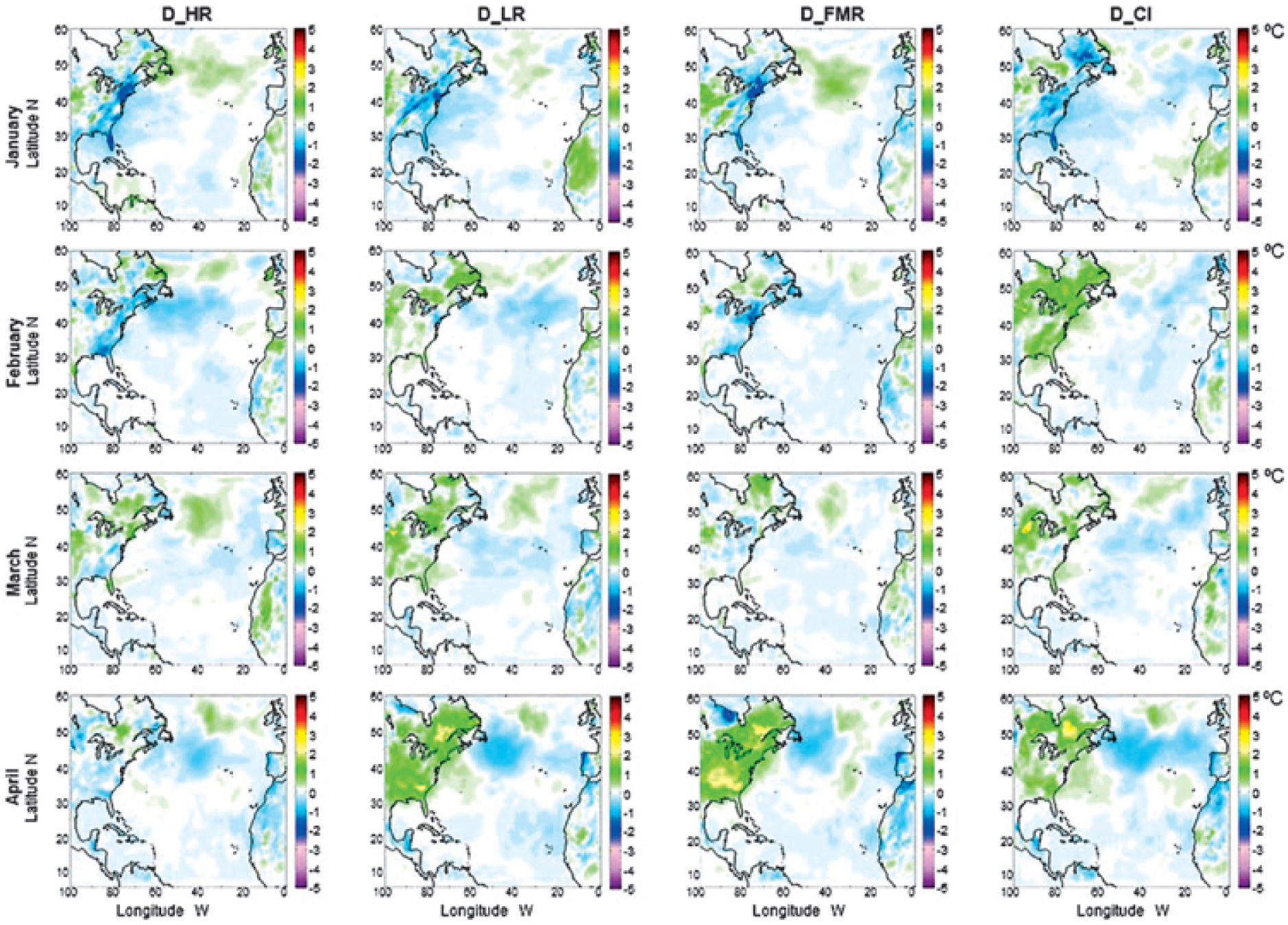
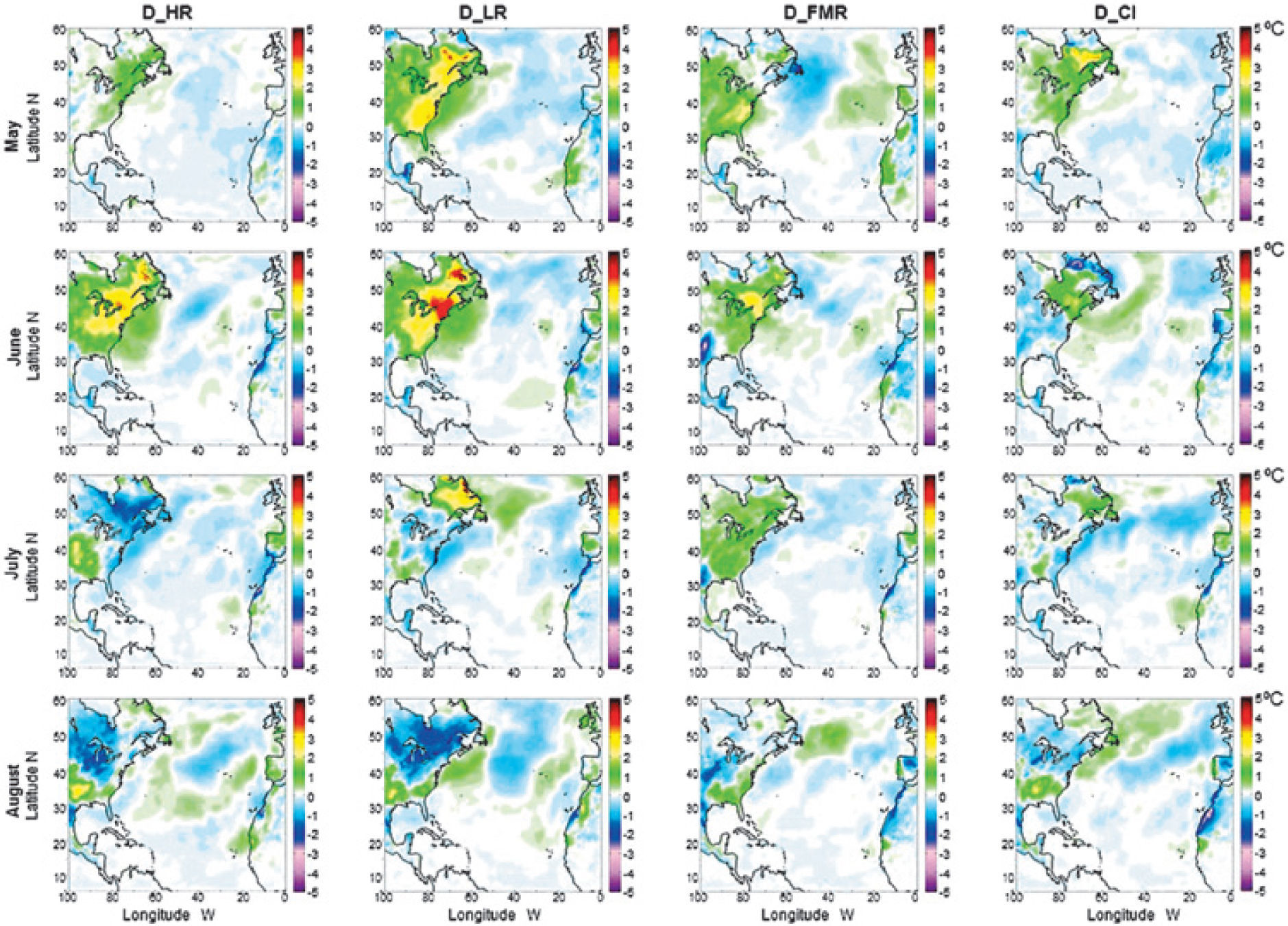
ResultsThe monthly mean surface temperature differences (D_HR, D_LR, D_FMR and D_IC), from September 1983 to August 1984, for each simulation are shown in figures 2, 3 and 4. Larger changes occur in latitudes higher than 30°N. The changes are observed on the Eastern US and Canada and Northwest Africa. In low latitudes (5°- 10°N) the differences are smaller compared to those observed at higher latitudes. Larger positive differences occur in November and June on the Eastern US and Canada and negative differences, also in November, occur on Northwest Africa.
In these plots, variations of surface temperature are noticeable for each case during the year of study. However, the variations observed for D_HR, D_LR and D_FMR are of the same magnitude as those corresponding to variations in the initial conditions D_IC. Then to determine if the model is more sensitive either to TSI changes or to changes in the initial conditions, we use the technique of dimensionless parameters.
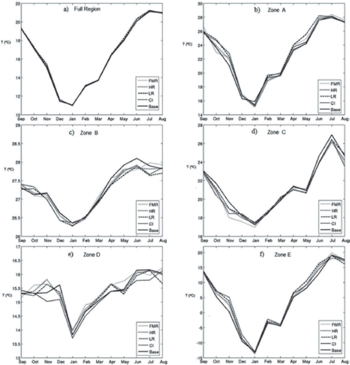
In Figures 2-4 we also see variations in some continental zones in low latitudes. Those changes are usually smaller than in higher latitudes. When we calculate the monthly surface temperature averaged over the full area of study (see Figure 5a), i.e. the simulation grid, the five simulations do not show meaningful differences; i.e. the base, HR, LR and FMR have the same monthly mean temperature over the full grid. This can be due to the fact that the zones where there are large differences are small compared to the zones where the differences are smaller. If we compute the monthly average for each one of the five zones (A, B, C, D and E) we found larger monthly differences. For instance in zones A, C, D and E there is a difference of at least 1°C in November and June, while in January and March the differences are smaller (see figs. 5b, 5d, 5e and 5f).
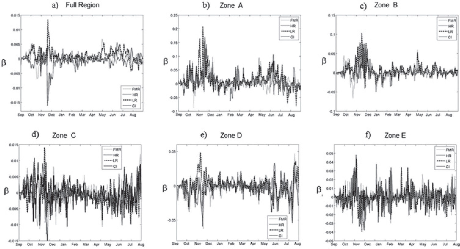
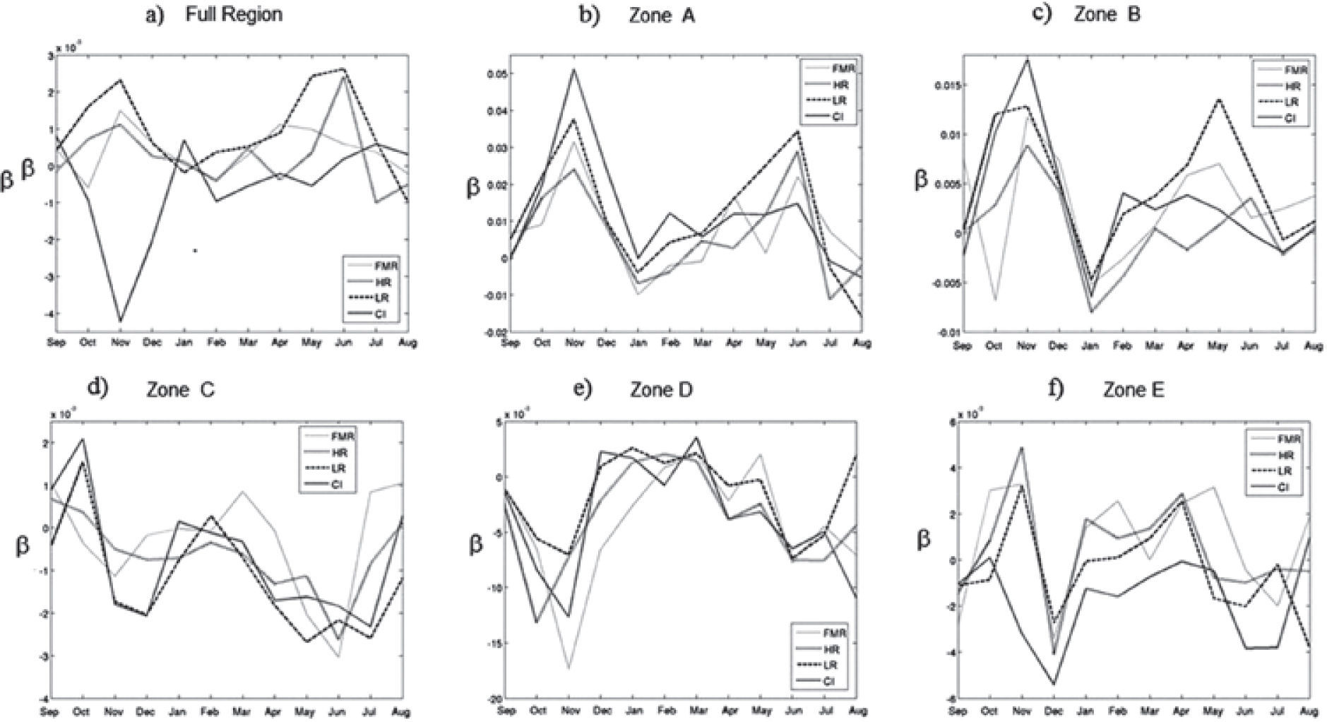
To quantify these differences the daily and monthly temperature sensitivity of the WRF model to changes in TSI using Equation (5) was computed. To calculate the daily sensitivity (Figure 6) over the area of study (Figure 5a) and the five zones (Figures 5b to 5f), we use T_0 as the base year daily average temperature of the area, and T as the daily average temperature in the area for the different TSI values. Also, the monthly temperature sensitivity over the area of study (Figure 7a) and the five zones (Figures 7b to 7F) was computed; here T_0 is the base year monthly average temperature and T is the monthly average temperature in the area for the different TSI values. In Figures 6 and 7, the curves for the various numerical experiments are different. Although the variations are small we notice that the temperature was more sensitive in November and June as we also notice in Figures 2 to 4. The average sensitivity of the temperature for each of the simulations is shown in Table 2. Figures 6 and 7 show that the sensitivity is positive for the various TSI, but it is negative for changes of initial conditions during November and June.
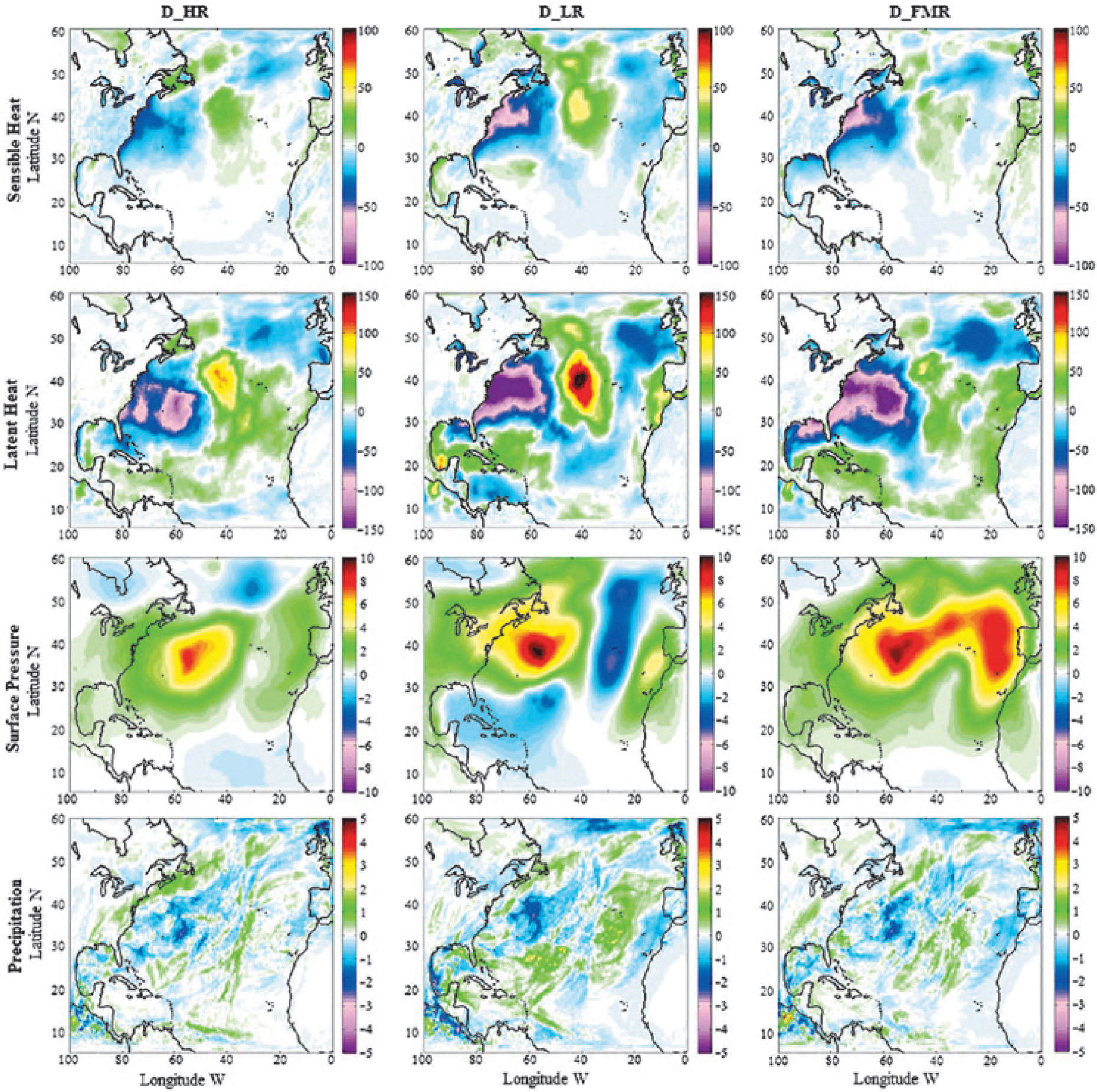
Finally, to complement the analysis made for the temperature, although is not the main purpose of this article to do a comprehensive analysis of all the variables that are available from the numerical simulations, we present results of: latent heat, sensible heat, surface pressure, and precipitation. Figure 8 shows the monthly average differences between the HR, LR and FMR and the base year, those are D_HR for HR-Base, D_LR for LR-Base and finally D_FMR for FMR-Base, respectively of the variables mentioned above (Cipagauta et al., 2013). Since our temperature analysis reveals that the month of November 1983, has larger differences with respect to the base year, we restrict the presentation of the results of the additional variables to this month. These results show that changes in the TSI modify the temperature as well as other variables. Figure 8 shows that the largest changes in these variables also occur at higher latitudes. Changes of latent heat, sensible heat, and surface pressure occur mainly in the ocean rather than in the continents.
ConclusionsBased on predictions of GCM and the supposition of linearity, it was expected that an increase (decrease) in TSI would cause an increase (decrease) in surface temperature. However, Figures 2 to 4 show that this is not the case, for instance, in November and June for the three different values of TSI the temperature in Northeast EU and Canada increases, but the temperature change is larger for the FMR, while in Northwest Africa for the three scenarios of TSI there is a decrease in temperature, being larger during the FMR. Some studies using GCM suggest that some regions of the Earth´s surface could cool and others could heat by least 1°C as a results of changes caused by the differential heating of the land and ocean [Haigh et al., 2005; Meehl et al., 2008; Barriopedro et al., 2008; Lee et al.,2008]. Our results seem to support this suggestion.
However, temperature variations observed in the numerical experiment IC, are similar to those that occurred in experiments in which the TSI was varied, in the sense that the changes are observed in the same zones and of the same order of magnitude. However, the calculated model sensitivity shows that the sign corresponding to the TSI variations is opposite to the sign of the change in initial conditions (Figure 6a, 7a). This would suggest that in this model the temperature changes observed due to different conditions of TSI are different from variations in the IC. Although we have only one IC experiment, this gives an idea of the order of magnitude expected for the differences that can be found for a small change in the initial conditions.
Therefore, we conclude that changes in TSI produce changes similar to those of a disturbance in the initial conditions, but do not lead to significant changes in the conditions of the average temperature. Probably significant temperature variations will be produced if larger TSI changes occurred. To have more conclusive results concerning the sensitivity of the model to TSI variations leading to effects on weather, it will be desirable to couple the WRF model with an ocean model in order to allow the ocean heat content change under different TSI conditions. Our results are relevant for climate change experiments using the technique of downscaling [Giorgi et al, 2009] because it highlights the importance of using coupled ocean-atmosphere models to get a better temperature setting.


