This work presents a practical method for estimating the full kinematic state of a vehicle, along with sensor error parameters, through the integration of inertial and GPS measurements. This kind of system for determining attitude and position of vehicles and craft (either manned or unmanned) is essential for real time, guidance and navigation tasks, as well as for mobile robot applications.
The architecture of the system is based in an Extended Kalman filtering approach in direct configuration. In this case, the filter is explicitly derived from the kinematic model, as well as from the models of sensors error. The architecture has been designed in a manner that it permits to be easily modified, in order to be applied to vehicles with diverse dynamical behaviors.
The estimated variables and parameters are: i) Attitude and bias-compensated rotational speed of the vehicle, ii) Position, velocity and bias-compensated acceleration of the vehicle and iii) bias of gyroscopes and accelerometers. Experimental results with real data show that the proposed method is enough robust for its use along with low-cost sensors.
The process for autonomously estimating the state of a vehicle (e.g position, velocity, orientation, etc.), while it is maneuvering along a trajectory, is often referred as navigation.
The autonomous navigation is an important capability for both manned and unmanned vehicles. In our context the term “autonomous” refer to the capacity of the system for estimating the state of the vehicle without the aid of a human operator. Often, the autonomous navigation is a prerequisite for control tasks.
The Inertial Navigation System (INS) is one of the most widely used dead reckoning systems. A typical INS fuses sensory information taken from inertial sensors (accelerometers) and rotational sensors (gyroscopes) in order to continuously estimate position and orientation of the body (vehicle). Because different sources of sensor errors are integrated over time, an INS can provide correct and high frequency (typically in the range of 100 to 200Hz) information but only for short term. This fact is especially notorious when lowcost sensors are used. On the other hand, a Global Positioning System (GPS) provides globalreferenced position and velocity estimations at low rate (typically in the range of 1 to 4Hz). The integration of both systems (INS and GPS) can generate a navigation system capable of exploiting the advantages of both, and also limits the drawbacks of the systems viewed by separate. Thus, a GPS-aided INS can produce estimates of the full state of the vehicle, both at high frequency as drift-free.
The integration of inertial sensors with GPS is broadly classified as follows [25]:
- •
Loosely coupled system.
- •
Tightly coupled system.
- •
Ultra-tightly coupled system
In loosely coupled systems [8–13], [16], [18] and [19], the GPS data (e.g. position velocity, etc) are fused explicitly with INS data. This kind of systems is significantly dependent on the availability of GPS data.
In tightly coupled systems [6] and [13], the GPS raw measurements (e.g pseudo ranges) are fused directly with the INS data. The main advantage of this kind of methods is that the system can carry out GPS measurement updates, even if there are less than four satellites available. Their downside has to be with the increase of complexity.
In Ultra-tightly coupled systems [26], the INS output (position, velocity and attitude) is used as an external input to the GPS receiver. The INS output aid in prepositioning calculation for faster signal acquisition and in interference rejection during signal tracking. The implementation of this kind of systems is often complicated because access to the GPS's firmware is required.
Different techniques of state estimate have been used for integrating INS and GPS. Schemes presented in [1] and [2] are based in techniques of linear Kalman filtering. The Kalman filter (KF), commonly used in estimating the system state variables and suppressing the measurement noise, has been recognized as one of the most powerful state estimation techniques. The KF allows to merge information obtained from different sensor sources in a structured manner. For example in [29], a KF- based method for estimating position is presented, this approach combines visual data with wireless sensors network information. Commonly methods based on linear filtering utilize simplified (linearized) models. Thus, some computational time is saved, but at the cost of some decrease in performance. However, the wide variety of processing devices currently available makes feasible the implementation of complex algorithms in order to improve performance.
Due to the nonlinear nature of the problem, the nonlinear version of the Kalman Filter (The Extended Kalman Filter or EKF) has been the technique typically used to compute the GPS-INS solution. There are two basic ways for implementing the EKF:
- •
Indirect formulation.
- •
Direct formulation.
The EKF in Indirect formulation (also referred as the error state space formulation), estimates a state vector which represents the errors defined by the estimated state and the estimated nominal trajectory. An error model for each component of the state is needed in order to estimate the measurement residual. The measurement in the error state space formulation is made up entirely of system errors and is almost independent of the kinematic model. Most of the approaches found in literature are based in this kind of configuration [3–13].
The EKF in Direct configuration (also referred to as total state space formulation) updates the vector state implicitly from the predicted state and the measurement residual (the difference between the predicted and current measurement).
In this kind of EKF configuration, the system is essentially derived from the kinematics. One of the characteristics of the direct configuration is its conceptual clarity and simplicity. A review on the EKF and its configurations can be found in [14].
In addition, it is possible to find others methods which rely in some variations of Kalman filtering as: Adaptative Kalman filtering [15], Unscented Kalman filtering [16]. Particle filtering (PF) is a nonlinear estimation technique which has been also utilized for integrating INS and GPS. The advantage of PF is the capability to deal with nonlinear non-Gaussian models. Some methods based on PF are [17] and [18]. Another kind of methods relies in estimation techniques coming from the artificial intelligent (Al) research community, as [19], which is based on Neural Networks. Alternatively, there is also possible to find hardware-oriented approaches as [20].
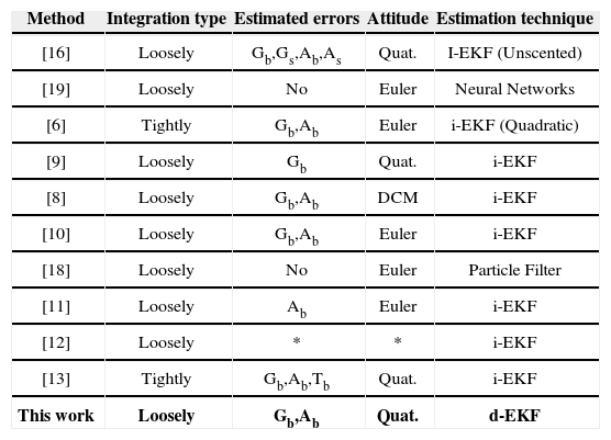
Table I presents a resume of some methods published in journals in recent years. The characteristics of the methods presented in Table I are: i) Integration type, ii) estimated parameters of sensors error (e.g. bias, scale, etc.) iii) attitude representation, and iv) main estimation technique. While it is possible to find different families of approaches in literature, the EKF is still the standard estimation technique used for GPS-aided Inertial Navigations Systems. Nevertheless, the use of the EKF in direct configuration has been much less explored than its counterpart; the EKF in indirect configuration (See Table I). This is especially the case when sensor errors (e.g. bias of gyros and accelerometers) want to be included in the estimated vector state.
Resume of Methods. *Not specified. For “Estimated errors” column: G = gyroscope, A = accelerometer, T = GPS time, b = bias, s = scale, (e.g. Gb means gyro bias). For “Attitude” column: DCM means Direction Cosine Matrix, and Quat. is the abbreviation of quaternion. For “Estimation Technique” column, i-EKF = Extended Kalman Filter in indirect configuration, d-EKF = Extended Kalman Filter in direct configuration. In parentheses are indicated.
| Method | Integration type | Estimated errors | Attitude | Estimation technique |
|---|---|---|---|---|
| [16] | Loosely | Gb,Gs,Ab,As | Quat. | I-EKF (Unscented) |
| [19] | Loosely | No | Euler | Neural Networks |
| [6] | Tightly | Gb,Ab | Euler | i-EKF (Quadratic) |
| [9] | Loosely | Gb | Quat. | i-EKF |
| [8] | Loosely | Gb,Ab | DCM | i-EKF |
| [10] | Loosely | Gb,Ab | Euler | i-EKF |
| [18] | Loosely | No | Euler | Particle Filter |
| [11] | Loosely | Ab | Euler | i-EKF |
| [12] | Loosely | * | * | i-EKF |
| [13] | Tightly | Gb,Ab,Tb | Quat. | i-EKF |
| This work | Loosely | Gb,Ab | Quat. | d-EKF |
This paper describes a novel method for implementing a GPS-INS integrated system. The proposed system architecture is based in an Extended Kalman filtering approach in direct configuration. Thus, the filter is explicitly derived from the kinematic model as well as from the models of sensors error.
The paper is organized as follows: Section II describes in detail the proposed method. In section III experimental results, carried out with real data, are presented in order to validate the performance of the proposed method. Finally section IV presents conclusions and final remarks.
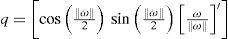
2Method description2.1Vector state and system specificationThe goal of the proposed method is the estimation of the following system state x¿:
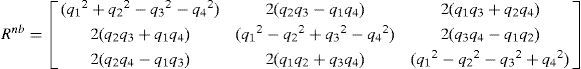
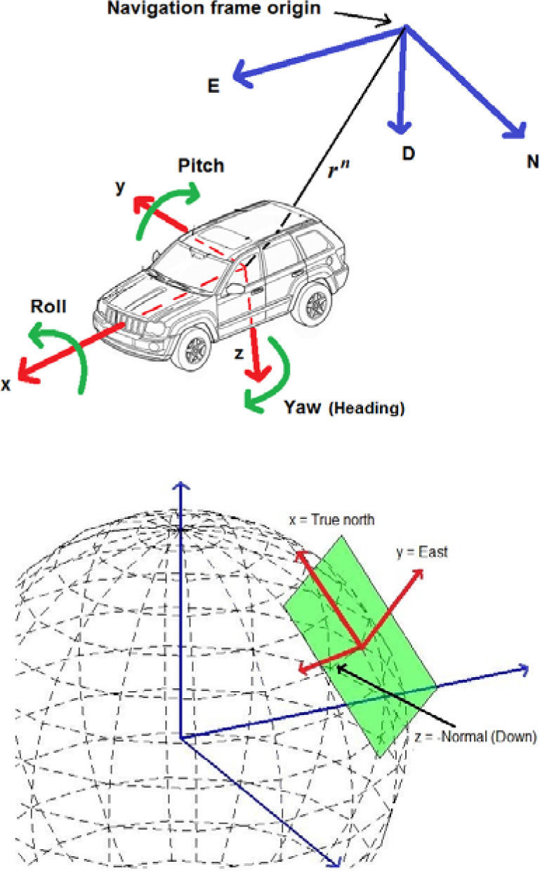
where qnb = [q1,q2,q3,q4] is a unit quaternion representing the orientation (roll, pitch and yaw) of the body (vehicle). ¿b = [¿x¿y¿z] is the biascompensated velocity rotation of the body expressed in the body frame (b). xg = [xg_x xg_y xg_z] is the bias of gyros. rn = [xvyvzv] represents the origin of the body coordinate frame (b) expressed in the navigation frame (n). vn = [vx vy vz] is the velocity of the body expressed in the navigation frame. An = [axayaz] represents the bias-compensated acceleration of the body expressed in the navigation frame. xa = [xa_x xa_y xa_z] is the bias of the accelerometers. Figure 1 (upper plot) illustrates the relation between the vehicle (body) frame and the coordinate systems used as navigation frame.
. The local tangent frame is used as the navigation frame (lower). For navigation in a local tangent frame, the origin of the ned coordinate axes would be at some convenient point near the area of operation.")
Relation between the vehicle frame and the coordinate system used as navigation frame (upper). The local tangent frame is used as the navigation frame (lower). For navigation in a local tangent frame, the origin of the ned coordinate axes would be at some convenient point near the area of operation.
The proposed method is mainly intended for local autonomous vehicle navigation. Thus, the local tangent frame is used as the navigation frame (n) (Figure 1, lower plot). In this work, the axes of the coordinate systems follow the NED (North, East, Down) convention.
In order to estimate the system state x¿ two kinds of measurement are considered:
a)High rate measurementsAn inertial measurement unit (IMU) of 9DOF formed by i) 3-axis gyroscope, ii) 3-axis accelerometer, and iii) 3-axis magnetometer, is considered. See [27] for an extended discussion about estimating orientation using a 9DOF IMU. Whereas magnetometers are used only for the system initialization, it is assumed that at every k steps there is availability of gyros and accelerometers measurements.
Gyroscopes measurements: the angular rate ¿b of the vehicle, measured by the gyros (in the body frame) as yg, can be modeled by:
where xg is an additive error (bias) and vg is a Gaussian white noise with power spectral density (PSD) ¿g2.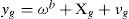
Accelerometer measurements: the acceleration of the vehicle ab, measured by the accelerometers (in the body frame) as ya can be modeled by:
where, gb is the gravity vector expressed in the body frame, xa is an additive error (bias), and va is a Gaussian white noise with PSD ¿a2.b)Low rate measurements: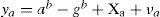
GPS measurements of position zr and orientation z¿, available at n*k steps, can be modeled by:
where rn = [xvyvzv] represents the position of the GPS antenna expressed in the navigation frame (in Cartesian coordinates), and vr is a Gaussian white noise with PSD ¿r2. ¿n is the course angle of the vehicle, measured by the GPS unit (respect to the geographic north), and v¿ is a Gaussian white noise with PSD ¿¿2. See [28] for an extended discussion about GPS measurement models. Commonly, position measurements are obtained from GPS devices in geodetic coordinates (latitude longitude height). If this is the case, the GPS position measurements must be transformed to their corresponding local tangent frame coordinates.2.2Architecture of the system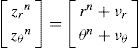
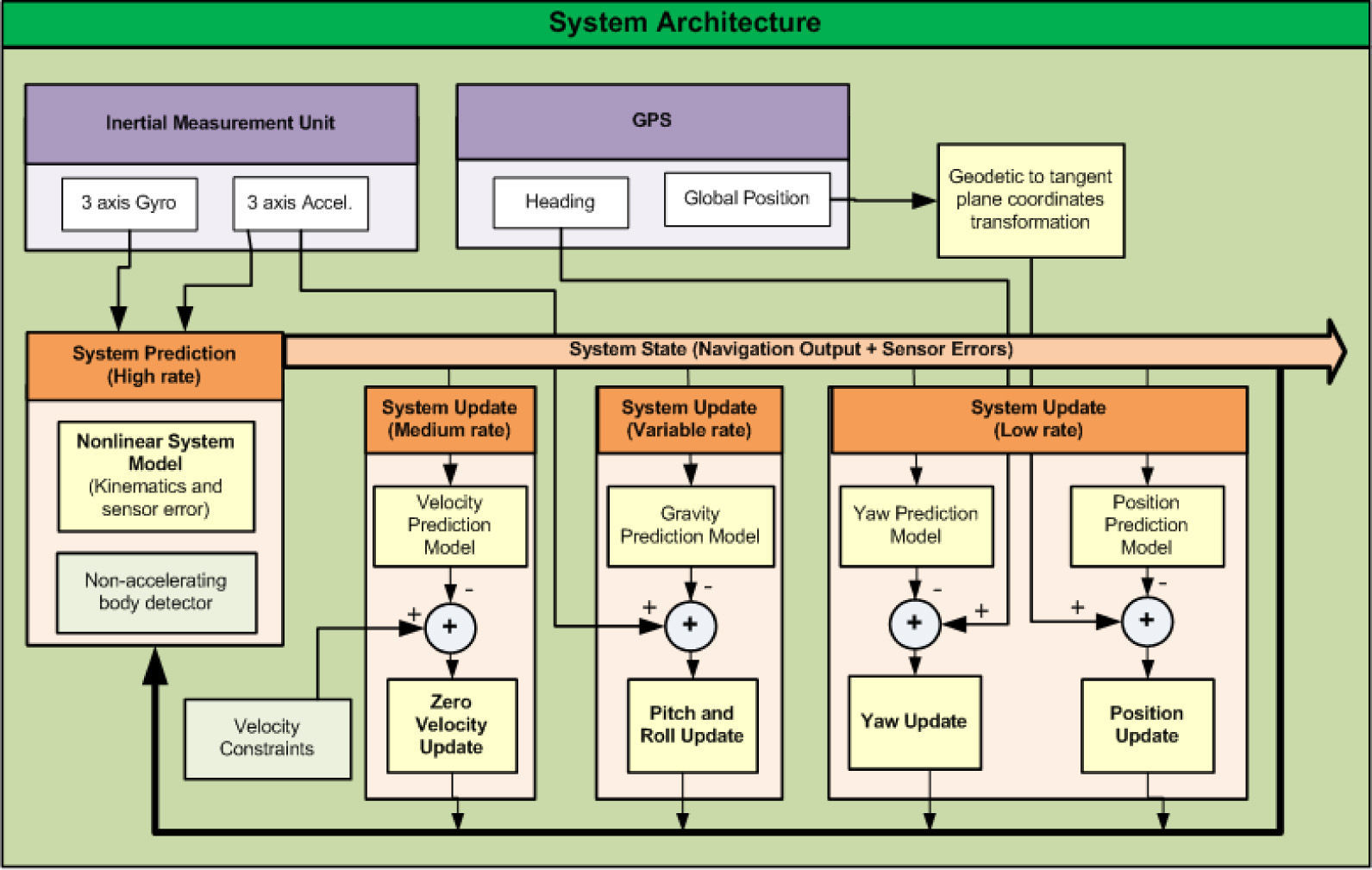
The architecture of the system is based in the typical loop of prediction-update steps, defined by an EKF in direct configuration (Figure 2).

System Prediction: Prediction equations propagate in time the estimation of the system state, by means of the measurements obtained from gyros and accelerometers. Prediction equations offer correct estimates at high frequency, but only for short term.
System Updates: In order to correct and limit the drift in estimates of the system state, globally referenced information along with a priori assumptions about the systems dynamics, are fused into the system, by means of the update equations. Three kinds of system updates are considered:
- •
Updates by means of dynamical constraints: apriori knowledge about the vehicle dynamics is incorporated into the system at medium rate.
- •
Updates by means of the observation of the gravity vector: information about the attitude of the vehicle (roll and pitch) is incorporated into the system at variable rate.
- •
Updates by means of GPS measurements: information about position and heading of the vehicle are incorporated into the system at low rate.
At every k step that measurements of gyroscopes and accelerometers are available, the system state is taken a step forward by the following (discrete) nonlinear model:
being q(Rbn [¿b ¿t]′) a quaternion computed from the rotation vector Rbn[¿b¿t]′ (using Eq. 25). The rotation vector [¿b¿t] is determined by the bias-compensated gyro readings ¿b. Note that [¿b ¿t] is converted to navigation coordinates via the body-to-navigation rotation matrix Rbn. The matrix Rbn is computed from the current quaternion qnb, (using Eq. 26). A similar model for integrating attitude by means of gyro measurements was used in previous author work [21].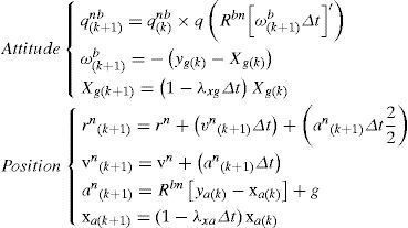
Parameters ¿xg and ¿xa are correlation time factors which respectively model how fast the bias of gyro and accelerometers are varying. gis the gravity vector and ¿t, the sample time of the system.
The state covariance matrix P is taken a step forward by:

The measurement noise of gyroscopes and accelerometers (respectively vg and va) are incorporated into the system by means of the process noise covariance matrix U, throughparameters ¿g2 and ¿a2:

The full model used for propagating the sensor bias error is: biask+1 = (1−¿¿t)biask + vb. Where vb models uncertainty in bias drift. The uncertainty in bias for gyro and accelerometers (respectively vxg and vxa) is incorporated into the system through the noise covariance matrix U via PSD parameters ¿xg2 and ¿xa2.
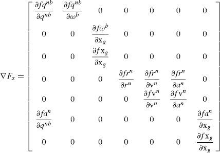
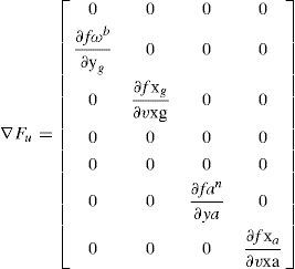
The Jacobian ∇Fx(Eq. 8) is formed by the partial derivatives of the nonlinear prediction model (Eq. 5) with respect to the system state x¿. In Jacobians the notation “∂fx/∂y” is used for partial derivatives. And it reads as the partial derivative of the function f (which estimates the state variable x), with respect to the variable y. Jacobian ∇Fu (Eq. 9) is formed by the partial derivatives of the nonlinear prediction model (Eq. 5) with respect to the system inputs.
In Jacobian ∇Fx, it can be observed that the only term that correlates attitude and position equations (see Eq. 5) is: ∂fan/∂qnb. Therefore:
- •
∂fan/∂qnb≠ 0 couples attitude and position estimation.
- •
∂fan/∂qnb= 0 couples attitude and position estimation
One of the implications of coupling attitude and position equations is: If one of the axis of the IMU (usually the x axis) is assumed to be aligned (fixedly) toward the displacement of the vehicle (as it occurs in a typical land-vehicle configuration), then GPS position measurements can be used for updating attitude. However, there are some cases where the assumption described above does not apply. For example, this is the case of an airplane where the pitch angle does not coincide with the flight path angle due to the angle of attack. In this work it is assumed that attitude and position equations are coupled (∂fan/∂qnb ≠ 0).
2.4System updateEvery time that is needed, the filter can be updated as follows:
where zi is the current measurement and hi=hx¿ is the predicted measurement. W is the Kalman gain computed from;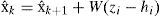
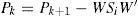
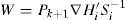
Si is the innovation covariance matrix
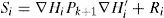
∇Hi is the Jacobian formed by the partial derivatives of the measurement prediction model h(x¿) with respect to the system state x¿. Ri is the measurement noise covariance matrix. Equations 10 to 13 are either used for each one of the system updates that are carried out, along with their corresponding: i) zi ii) hi, iii) ∇Hi, and iv) Ri.
a)Dynamical constraints updateKnowledge about the vehicle dynamics can be incorporated into the system through the filter updates [22]. For this work, the data used for experiments was captured by measurement devices mounted over a land vehicle. In this case, nonholonomic constraints are included in the system in the form of zero velocity updates.
If axis x of the IMU is assumed to be aligned with the axis x of the land vehicle, then y and z velocities (in the body frame), respectively vyb and vzb can be modeled as zero plus an additive Gaussian white noise vv with PSD ¿v2.
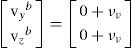
The measurement prediction hv0 is computed from:
were
Rnb is the navigation to body rotation matrix computed from the current quaternion qnb, and vn is the velocity of the vehicle (expressed in the navigation frame) obtained from the current vector state x¿
For updating the filter (Equations 10 to 13):
b)Roll and pitch updates
If the vehicle is not accelerating, (i.e.ab ≈ 0) then Eq. 3 can be approximated as ya ≈ gb+va(neglecting or estimating xa). In this situation, accelerometers measurements ya provide noisy observations (in the body frame) about the gravity vector. The gravity vector g can be used as an external reference for correcting roll and pitch estimations [21].
In order to detect k instants, where the body is in a non-accelerating mode, the Stance Hypothesis Optimal Detector (SHOE) is used [23]
The gravity vector g is predicted to be measured by the accelerometers as hg:
where gc is the constant gravity and Rnb is the navigation to body rotation matrix computed from the current quaternion qnb. For updating the filter(Equations 10 to 13):(c)Position and heading updates

In this work, a loosely coupled approach is used for incorporating the data provided by the GPS unit into the system state. In a loosely coupled approach, the high level outputs provided by the GPS unit are directly incorporated into the system state via their corresponding measurement prediction model.
On the other hand, the architecture proposed in this work could be extended in order to be suitable for a tightly coupled approach. Among other things (as the use of an adequate measurement model), in order to implement such adaptation, the system state should be augmented for including GPS errors (e.g. time bias).
The model hr used for predicting the GPS measurements about the vehicle position is:

For updating the filter (Equations 10 to 13):

In order to update the vehicle yaw using GPS measurements, it is assumed that the heading (yaw) of the vehicle is fixed with respect to the angle, of course, measured by the GPS. If the above assumption is not valid, as it could be the case for some aerial vehicles (e.g. helicopter), then an external reference should be used for updating the yaw (e.g. earth's magnetic field).
The model h¿ used for predicting the angle of course measured by the GPS is:
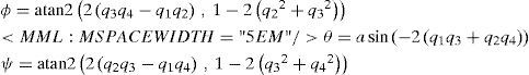
where qnb=[q1,q2,q3,q4] is the current quaternion. For updating the filter (Equations 10 to 13):

Position and heading updates can be also implemented together in a single filter update step.
2.5System initializationThe system is initialized as follows:
where ¿ is an arbitrary very small positive value. The initial attitude q2ininb and its corresponding initial uncertainty ¿qnbini2 are estimated in the same manner as [27]. It is important to remark that in this work, magnetometers are used only for having an initial estimation of heading (yaw)
In Eq. 23, note that the initial position of the vehicle is set to zero due to the fact that local tangent plane is used as navigation frame. On the other hand, for transforming GPS measurements, from geodetic coordinates to the tangent plane coordinates, it is necessary to know the geographic location of the tangent plane origin.
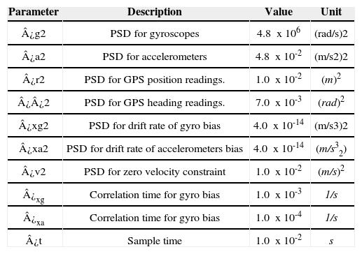
3Experimental resultsIn order to test the performance of the proposed method, a MATLAB© implementation of the method was executed off-line using the Malaga dataset [24] as input signals. The Malaga dataset is freely available online, and contains several sources of sensors signals along with an accurate ground truth. The inertial measurement data were collected at 100Hz, whereas GPS data were collected at 4Hz. The measurements devices, used for collecting the data, were mounted over an electric buggy-type vehicle, (see [24]). Table II shows information about the parameters used in experiments.
Parameters.
| Parameter | Description | Value | Unit |
|---|---|---|---|
| ¿g2 | PSD for gyroscopes | 4.8 x10⁶ | (rad/s)2 |
| ¿a2 | PSD for accelerometers | 4.8 x10⁻² | (m/s2)2 |
| ¿r2 | PSD for GPS position readings. | 1.0 x10⁻² | (m)2 |
| ¿¿2 | PSD for GPS heading readings. | 7.0 x10⁻³ | (rad)2 |
| ¿xg2 | PSD for drift rate of gyro bias | 4.0 x10⁻¹⁴ | (m/s3)2 |
| ¿xa2 | PSD for drift rate of accelerometers bias | 4.0 x10⁻¹⁴ | (m/s32) |
| ¿v2 | PSD for zero velocity constraint | 1.0 x10⁻² | (m/s)2 |
| ¿xg | Correlation time for gyro bias | 1.0 x10⁻³ | 1/s |
| ¿xa | Correlation time for gyro bias | 1.0 x10⁻⁴ | 1/s |
| ¿t | Sample time | 1.0 x10⁻² | s |
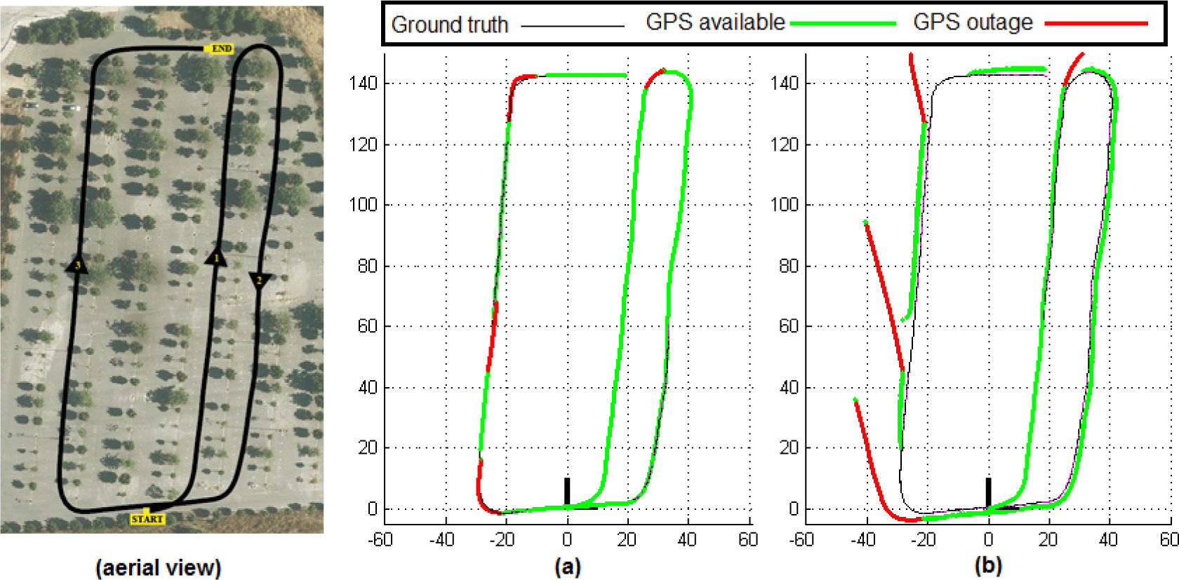
Figure 3 shows some of the experimental results obtained from the input signals that have been described above. The left graphic, shows an aerial view of the path followed by the vehicle as well as its environment. Plot (a) shows the trajectory estimated by the proposed method.
, shows its corresponding estimated trajectory. Green segments indicate periods of time with GPS availability. Red segments indicate periods of time where GPS outages occur. Plot (b) shows the trajectory obtained when the parameters of the sensors error (xg and xa) are ignored.")
Left plot: Aerial view illustrating the path followed by the vehicle, while the sensor data were collected. Plot (a), shows its corresponding estimated trajectory. Green segments indicate periods of time with GPS availability. Red segments indicate periods of time where GPS outages occur. Plot (b) shows the trajectory obtained when the parameters of the sensors error (xg and xa) are ignored.
In experiments some GPS outages were simulated in order to test the performance of the method for periods where navigation is solely based in inertial measurements (in the original dataset, the GPS signal is available for the whole trajectory). In Figure 3 (plots a and b) observe that the estimated trajectory is composed for green and red segments. Green segments indicate periods of time where GPS is available, whereas red segments indicate periods of time where GPS outages occur.
In order to validate the capability of the method for estimating the parameters of sensors error, the algorithm was executed again. In this case, running over the same input signals and conditions (GPS outages), but ignoring both, the estimated gyro bias xg and the estimated accelerometer bias xa. Plot (b) shows the adverse effects in the estimated trajectory, when sensor errors are ignored. In this case, and as it could be expected, there is a huge drift in the estimated trajectory for the periods of inertial navigation, where GPS is not available. Therefore, by comparing plots (a) and plot (b), it can be deduced that the method is performing the parameter estimation tasks reasonably well.
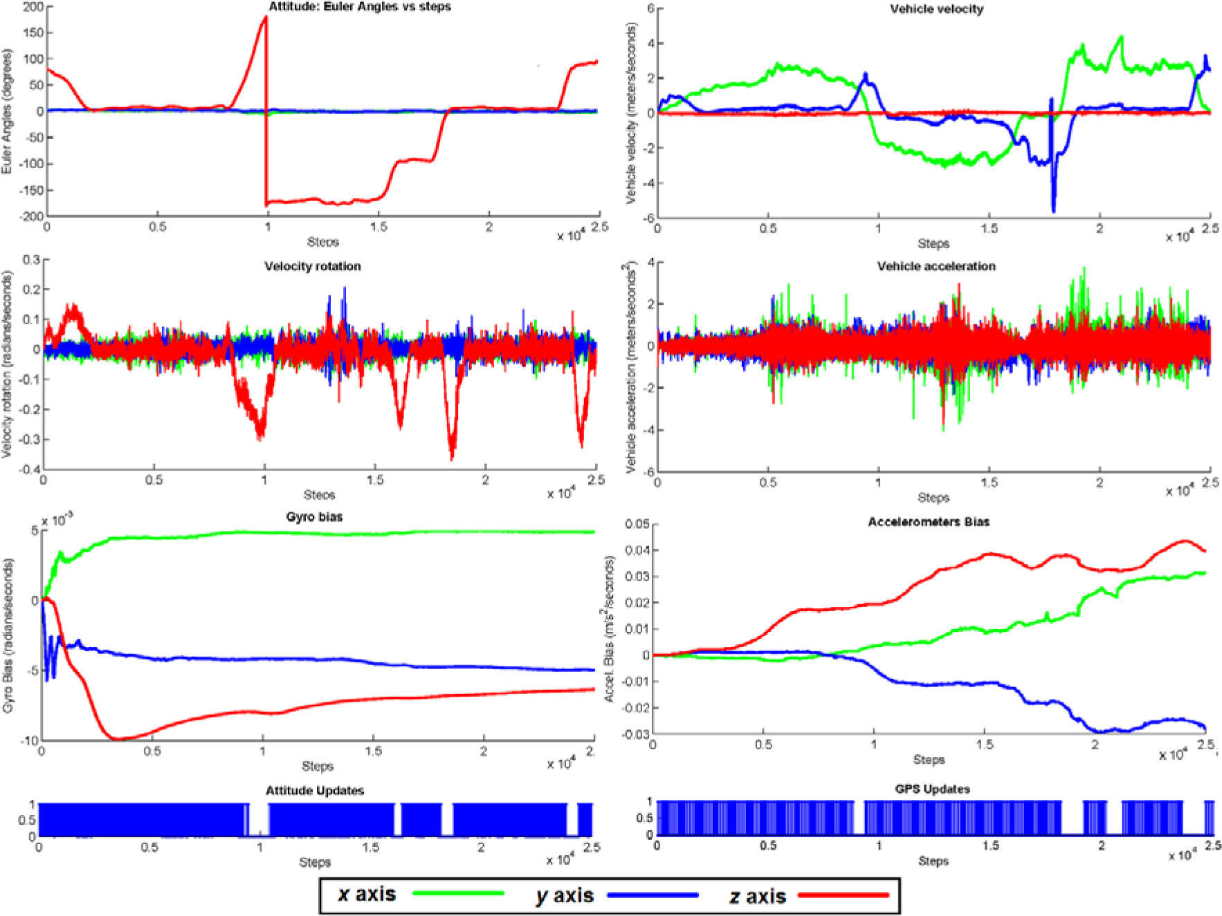
Figure 4. shows the progression over time for the rest of the estimated vector state of the vehicle [qnb, wb, xg, vn, an, xa], for the experiment executed with the full method (Fig. 3 (a)).
 Attitude of the vehicle qnb (expressed in Euler angles), b) Velocity rotation of the vehicle ¿b (expressed in the body frame b), c) Gyroscopes bias xg, d) Velocity of the vehicle vn (expressed in the navigation frame n), e) Acceleration of the vehicle an (expressed in n), and f) Accelerometers bias xa. The lower plots illustrate periods where the attitude updates (left) and the GPS updates (right) occur.")
Estimation results for a) Attitude of the vehicle qnb (expressed in Euler angles), b) Velocity rotation of the vehicle ¿b (expressed in the body frame b), c) Gyroscopes bias xg, d) Velocity of the vehicle vn (expressed in the navigation frame n), e) Acceleration of the vehicle an (expressed in n), and f) Accelerometers bias xa. The lower plots illustrate periods where the attitude updates (left) and the GPS updates (right) occur.
The lower plots illustrate periods of time where attitude and GPS updates take place.
For this experiment, observe that attitude updates (roll and pitch) are suitably suspended when the vehicle is experimenting some sudden turns. The GPS outages can also be appreciated in the lower-right plot.
4ConclusionsThis work presents a practical method for estimating the full kinematic state of a vehicle, along with sensor error parameters, through the integration of inertial and GPS measurements. The estimated vector state is formed by 22 state variables: of which, 16 describes the full motion of the body in 6DOF, and 6 describes the parameters of sensors error (gyros and accelerometers bias). The architecture of the system is based in an Extended Kalman filtering approach in direct configuration. The EKF is still the standard estimation technique for this kind of systems. However, practically all recent approaches found in literature are based in the indirect configuration of the filter (called also error configuration).
One of the motivations of the proposed approach is due to the clarity and simplicity associated with the EKF in direct configuration. Moreover, the EKF in direct configuration is the approach typically taught in academic courses. In that sense, it is considered that the proposed method could be straightforwardly implemented, for example, by junior engineers and practitioners.
The proposed architecture has been also designed in a manner that permits the scalability of the system. For example, by means of the use of the adequate dynamical constraints (or possibly without them), the method could be easily modified for its use with another kind of vehicle or craft (e.g. aerial robots).
Different experiments with real data were carried out in order to validate the performance of the proposed method. The experimental results show that the method is capable of estimating the parameters of sensors error reasonably well.
Thereby, improving the system estimates in periods where GPS outages occur, and the navigation is based solely in inertial measurements.
Finally, it is considered that the method is enough robust for its use along with low-cost sensors.
Author wants to thanks to Jessica Davalos for its valuable support for correcting the language.