


The aim of this paper is to find solution for route planning in road network for a user, and to find the equilibrium in the path optimization problem, where the roads have uncertain attributes. The concept is based on the Dempster-Shafer theory and Dijkstra's algorithm, which help to model the uncertainty and to find the best route, respectively. Based on uncertain influencing factors an interval of travel time (so called cost interval) of each road can be calculated. An algorithm has been outlined for determining the best route comparing the intervals and using decision rules depending on the user's attitude. Priorities can be defined among the rules, and the constructed rule based mechanism for users’ demands is great contribution of this paper. The first task is discussed in more general in this paper, i.e. instead of travel time a general cost is investigated for any kind of network. At the solution of the second task, where the goal is to find equilibrium in transport network at case of uncertain situation, the result of the first task is used. Simulation tool has been used to find the equilibrium, which gives only approximate solution, but this is sufficient and appropriate solution for large networks. Furthermore this is built in a decision support system, which is another contribution of this work. At the end of the paper the implementation of the theoretical concept is presented with a test bed of a town presenting effects of different uncertain influencing factors for the roads.
In urban regions the transportation planning [1] is an existing problem, and an appropriate implementation process has great impacts. Lot of works deal with route choice (mostly for cars or vans, but for aircraft [3] as well), and navigation [4][5] in transportation area [2], and some of them take uncertainty into account as well, e.g. dealing with stochastic shortest path [6], using fuzzy [7] or two limit values [8] or neural networks [9]. Route planning problem and uncertainty can occur in many different networks, like electric power systems, telecommunication networks, water distribution, networks, and transportation systems, but this paper (especially from session 4.2) focuses on transportation. Every transportation company would like to find the routes that represent the minimum delivery cost [21]. Solution of this problem in stochastic network having variations in attributes is more complicated, but there are some papers with promising suggestions and applications [22].
There is a question in best path search: if every driver travelled on the base of his/her perceived best path, they may influence to each other; so will be this situation the best for all participants? Wardrop [12] has investigated this question and he has recognized alternative possible behaviours of users of transport networks, and stated two principles, which are commonly named after him:
- •
First principle: The journey times of all paths actually used are equal. These are equal or less than those which would be experienced by a single vehicle on any unused path.
- •
Second principle: The average journey time is minimal.
The first principle corresponds to the behavioural principle in which travellers seek to (unilaterally) determine their minimal costs of travel whereas the second principle corresponds to the behavioural principle in which the total cost in the network is minimal. Two kinds of optimized system can be distinguished according to Dafermos and Sparrow [23]: system-optimized (S-O) and user-optimized (U-O) transportation networks (the U-O network problem also commonly referred to in the transportation literature as the traffic assignment problem [13][14]). In the U-O network problem the users act unilaterally, in selecting their paths; and in the S-O network problem the users select paths according to what is optimal from a societal point of view, in that the total cost in the system is minimized. The user-optimized (U-O) network problem coincides with Wardrop's first principle, and the S-O network with Wardrop's second principle. Wardrop investigated the route planning in road network with many users without uncertainty. On the other side a route search algorithm for any individual driver was presented in a work [11] taking uncertainty into account, but a more complex model was needed.
The aim of the work presented in this paper was to investigate the route search with many users at case of uncertainty. Individual drivers are presented in more detailed with attitude and decision possibilities in this paper. Furthermore a decision support system is elaborated based on simulation helping tool that is able to solve the equilibrium problem. The novelty of the suggested solution procedure is that the equilibrium solving tool can handle intervals (so called cost intervals coming from uncertainty) instead of constant values, furthermore during the determination of the best route the users’ decision rules and priorities are considered.
2Related works to uncertaintyThe routing on a network is a general problem, as the users would like to find the best route with the smallest cost. In this paper a general solution is presented at first, where the network is represented by a graph and the cost may be any kind of cost of the edges in the graph (like length, number of steps, time, etc.) depending on the application area: biological network, computer, electrical, telecommunications, transport network. Then at the second part the focus is on the transport network with specially edge cost, namely the travel time. In this application area the routing can be user- or system-optimized; this paper presents a solution for both of them using a decision support system.
A network (represented by graph) is given with an ordered pair G: = (V, E) comprising a set V of vertices or nodes together with a set E of edges, which connect two nodes. The task is to reach a node from another in the graph at the smallest cost, where the costs of edges are given. Classical Dijkstra's [15] would give the shortest path in the graph with non-negative edge path costs, however this can handle only the certainty data. Therefore, a theory is needed that deals with uncertainty; and the Dempster-Shafer (DS) [16] is excellent solution for this, because it is able to handle the lack of the information also by belief functions [10].
In DS theory the set Ω = {H1, …, Hn} of all the possible states of the system, H1, … Hn still mutually exclusive. Let us denote by P(Q) the powerset 2Ω, and by A an element of P(Ω).
DS theory defines functions (m) called basic belief assignment (BBA) on the P(Ω).
Thus it enables to work with non-mutually exclusive pieces of evidence, represented by powerset P(Ω). The m(A) represents the proportion of evidence that the actual state belongs to A but there is no knowledge about evidence of subsets of A. Using DS theory a lower and an upper limit can be defined for the real probability of the evidence. The DS theory gives a solution for the combination of more basic belief assignment functions:
where m1,2 (ϕ) = 0 and K=∑A∩B=φm1Am2B
In previous work [11] based on probability intervals of DS theory we have defined the “cost interval” of edge instead of fix cost value. The cost interval is able to take the uncertainty of costs into account. The cost intervals can be calculated by the influencing factors – in case of more factors the combination of them can be calculated based on equation (3) – and these will give more sophisticated comparison possibility of different routes.
3User centric route planning model with uncertaintyRoute planning algorithm with uncertainty [11] is already solvedusing the cost intervals, and a large advantage of the procedure is the knowledge about dispersion (deviation) around the expected value of the received result. The algorithm gives the best sequences of the edges (best route), and the cost interval of this route, i.e. the expected value is between two boundaries: XMin, XMax:
During the algorithm there are many comparisons between the sub-routes, as candidates for further processing. The overall cost of any route (sub-routes or the route between the start and destination nodes) was the sum of the boundaries at cost intervals (Xi,Min and Xi,Max) of all edges (from 1 to n) of the route:
The deficiency of the algorithm was the restricted comparison of cost intervals of investigated routes, because only the unambiguous situations were evaluated correctly, the decisions of other comparisons were randomly.
In this paper a better solution is suggested, where the users can influence these decisions. One of the contributions of this work is the constructed rule based mechanism for users' demands; this session presents this mechanism in details.
Unambiguous situation is the non-overlapped cost intervals (XMax<YMin or another situation: YMax<XMin), and such overlapped intervals when one of them is definitely smaller (XMin<YMin and XMax<YMax orthe contrary) as can be seen in Fig 1.a. In these cases the decisions are unambiguous, the smaller should be chosen.

Unambiguous situation is the non-overlapped cost intervals (XMaxx<YMin or another situation: YMax<XMin), and such overlapped intervals when one of them is definitely smaller (XMin<YMin and XMax<YMax orthe contrary) as can be seen in Fig 1.a. In these cases the decisions are unambiguous, the smaller should be chosen.
- •
Pessimistic: If XMax< YMax, then interval X is considered as less; otherwise if XMax is not equal to YMax then interval Y is considered as less.
- •
Optimistic: If XMin< YMin, then interval X is considered as less; otherwise if XMax is not equal to YMax, theninterval Y is considered as less.
- •
Centralistic: If (XMin+XMax)/2 < (YMin+YMax)/2, then interval X is considered as less; otherwise if they are not equal to each other, then interval Y is considered as less.
- •
Risk avoider: If Xrange< Yrange, then interval X is considered as less; otherwise if they are not equal to each other then interval Y is considered as less (Xrange=XMax - XMin, Y = YMax - YMin).
- •
Comparative risk avoider: If Abs{YMax-XMax} >Abs{ (XMin+XMax)/2 – (YMin+YMax)/2 }, then the interval with smaller range(if Xrange< Yrange then choose interval X) is considered as less; where Abs(a) is the absolute value of a. In Fig. 1. at the examples b and d the interval X, and at the example c the interval Y should be chosen, respectively based on this rule.
The user can choose among them based on her/his risk attitude. Not only the decision rules, but priorities among them can be determined. For example the user can set that all comparisons should be based on (i) only the optimistic rule, or based on (ii) the optimistic and the centralistic rule. At latter case the priority should have been determined between optimistic and centralistic rule in the case when first rule gives tie result (e.g. if XMin = YMin, then the better alternative can not be decided at optimistic rules, so centralistic rule will help to choose the appropriate alternative). All basic rules can be used at the prioritization by sorting of them, moreover additional rules can be defined for this. Thus the constructed rule based mechanism will serve the user's demand. In the next session the equilibrium solution of more users' demands is discussed.
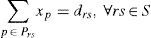
4Finding equilibrium for decision support4.1Optimization problemLet p denote a path consisting of a sequence of edges connecting an origin/destination (O/D) pair. Let Prs denote the set of paths connecting the origin r to destination s pair of nodes as described in Nagurney's paper [17]. Let S represent the set of origin/destination pairs of nodes, and let P denote the set of all paths in the network assuming that S is given. Let xp represent the flow on path p and let fe denote the flow on edge e. The following conservation of flow equation must be held:
where δep is equal to 1, if edge e is contained in path p, and 0, otherwise. Expression (7) states that the flow on an edge e is equal to the sum of all the path flows on paths p that contain (traverse) edge e. Let drs denote the demand associated with O/D pair rs, which should be the sum of the flows on different paths:
Let 1Ce denote the edge cost associated with traversing edge e for a user. Assume that the edge cost function is given by a separable function, furthermore this function is assumed to be continuous and an increasing function of the edge flow fe in order to model the effect of the edge flow on the cost.
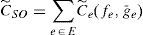
Let Ce denote the total cost of edge e for all users traversing this edge:

The total cost of the whole network is the sum of the all edge costs:
The system-optimization problem can be expressed by finding the minimum of CSO. The user-optimization problem is very similar, the constraint equations are identical in both of them, but the aim is different. The goal of the U-O problem is to minimize the following:
subject to (6)-(8).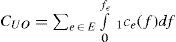
These optimization problems are related to constant cost values, but at uncertain case we can use intervals (so called cost intervals) discussed at the previous session. The costinterval of an edge depends on factors (in transport application area these factors can be the flow and on other influencing factors, like weather, actual lane numbers.). Let us define k different influencing factors: g1, g2, …, gk. The actual values of these factors for an edge e are: ge1, ge2, …, gek, briefly in vector format: ge
The cost interval of an edge for a user:
where the left expression is the minimal, the right one is the maximal value of the interval.
The total cost interval of an edge for all users:

The total cost interval of all edges for the whole network at the system-optimization and at the user-optimization problem, respectively:
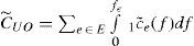
The left size of (23) and (24) are intervals; at both problems the aim is to minimize these costs. The users can choose rules in own defined priority order – as discussed at previous session – before the minimization procedure. A simulation method is presented for solving this minimization problem.
4.2Solution for finding equilibrium with simulationFor solving the problem described above so-called user-equilibrium program solution algorithms (e.g. the Frank–Wolfe algorithm) are well known. These theoretical algorithms are appropriate for small and average models, but not efficient for large networks. One possibility solution is the changing state in time [18], e.g. the time expansion of the spatial network is solved in work [19] by MILP (Mixed Integer Linear Programming), but this leads to a very large graph (the number of the nodes is the number of the original nodes multiplied by the number of the time steps).
Simulation tools can be also used to find the equilibrium, which give only approximate solution (but this tends to theoretical solution by increasing simulation run length), but capable for large networks.
The solution – for especially transport application area – presented in this paper is based on work [20] using simulation with an iterative procedure, which converges to the conditions mentioned above. The solution consists of two main components: a method to determine a new set of time-dependent path flows given the experienced path travel times (i.e. the previously used phrase “cost” is travel time from now on) on the previous iteration, and a method to determine the actual travel times that result from a given set of path flow rates. The latter problem is referred to as the “network-loading problem”, and can be solved using any path-based dynamic traffic model (e.g. INTEGRATION, CORSIM, AIMSUN2, VISSIM, PARAMICS, MITSIM). The iterative procedure furthermore requires a set of initial path flows, which are determined by assigning all vehicles to the shortest paths, based on free-flow conditions (details can be seen later at “Network loading”). The general structure of the procedure is shown schematically in Fig. 2, where the novelty comes from cost interval and user demands.

At the solution the inputs of the simulation model can be divided into three parts: static, dynamic and semi-dynamic. The static part contains the network structure with nodes, edges, cost functions, and the BBA functions (these can be declared based on statistics of reality) for network parameters (as can be seen the block “Network, BBA functions” in Fig. 2.). The dynamic part (“Facts”) of the input is unique for the given problem situation, so this consists of the actual facts about the circumstances. The semi-dynamic part contains the user demands (“User demands”) with chosen rules (from rule base) and origin destination pairs, which can change only by arrival of a new demand, but the demands are static during its serving.
The influencing factors of edges using uncertain probabilities are described by probability intervals. Based on these intervals the cost intervals of each edge (block “Cost-intervals”) can be calculated, so the network with parameter is given. The further part of the procedure takes the uncertain values of costs into account such a way.
The novelty of the solution procedure is that blocks “Determination paths” and “Network loading” should handle cost intervals instead of (constant) values, furthermore during the determination of paths the users' decision rules and priorities are considered.
The block “Demand ordering and optimization” of the procedure in Fig. 2 determines the order of the demands in the further execution, this order may influence the speed of the convergence. Without this the order of the demands is random, but the whole process may be faster by using optimization. The ordering optimization method tries to estimate the importance of the unique demands based on some features (e.g. how many other users would like to travel from the same origin to the same destination). This estimated importance can be used for ordering.
The block “Determination paths” of the procedure in Fig. 2 determines the paths in several iterations. In the first iteration the shortest (least cost) paths are based on free flow. At calculation for first demand the network is empty, then the edge costs are updated and the new shortest paths are computed for the second demand. The further calculations are similar, so this is repeated for all demands. At the end of the first iteration the network-loading (“Network loading”) is executed: this will be used for calculation the input flow for the next iteration.
Starting at the second iteration, and up to a prespecified maximum number of iterations, after each loading the edge costs are used to determine a new set of shortest paths (and path flows) that are added to the current set of paths (and path flows). In these iteration steps the flows (vehicles) effect on each other (and the flow in the next iteration will depend on capacity as well). At each iteration n the volume assigned as input flow to each path in the set is Xp/n, where xp is the calculated flow on path p in the previous iteration.
Since the network loading does not have an analytical form, there is no formal convergence proof for these iterations. The convergence criteria can be chosen from the known ones in the literature. This may be based on the computational time limit or maximum number of iterations. Instead of pre-specified maximum number of iterations the difference also can be used for investigation of termination. The actual difference is defined by difference between the calculated total cost and the total cost that would have been calculated if all vehicles had the cost equal to that of the current shortest path. If this difference would less than a predefined threshold, then the process will terminate.
4.3Decision support for traffic operatorThe calculated equilibrium can be compared with the actual situation, and predefined operational rules can be investigated. These operational rules, e.g. alerts are able to show that the necessity of intervention to the actual traffic.
The whole equilibrium calculation and if-then rules with suggested operations form the decision support system (DSS) can be seen in Fig. 3. The traffic operator can use this DSS to control the traffic if necessary.
5Test bed for the implemented system
The solution described above has been implemented in C programming language. In order to test the theoretical solution a test bed has been constructed for representing a little town. The test bed contains the road network of the city with more than four-thousand points. Based on this the user is able to observe the behavior of algorithm in realistic scenarios: he/she can see the drivers’ routes by MapInfo software.
MapInfo Professional is able to draw the maps quickly, to move the map parts, to display the map information, and to analyze the graphical relationships. MapBasic Professional program language, as the related module of the MapInfo, can be used for creating of own applications. By MapInfo the data can be analyzed not only in graphical format, but in diagram, histogram as well. The diagrams can be seen together with the maps and the tables.
The graph of the transport networks has contained 4111 nodes and 5443 edges. The file network.mid consists of 5443 rows for describing the network, so each row corresponds to an edge. A row stores 26 kinds of data, like quality of the road surface, which types of vehicles can travel on the road, what is the speed limit, etc. For the modeling the most relevant features are selected from 26 kinds of data:
- •
identity of the beginning point
- •
identity of the end point
- •
direction of the road
- •
average speed on the road
- •
number of the lanes
- •
length of the road
Different influencing facts (factors): weather, vehicle density and closed lane represented the uncertainty phenomena. (Naturally many other factors could be involved into the model, like delay of vehicles at signalized intersections, or slow-down at ambulance vehicle; so the model could be more complex.) Regarding the simplified situation, the above factors are binary variables: the values of the weather are satisfactory or unsatisfactory, the values of vehicle density are low or high and the values of a closed lane are yes or no. The basic belief assignment (BBA) functions were as follows: m1: unsatisfactory weather, m2: high vehicle density, m3: closed lane. Based on these the cost intervals can be calculated for all roads in the network, which is the input data for route planning.
The next figure (Fig. 4.) shows the graphical representation of the transport networks of the little town. The bald line represents the best route found by our solution for a user's demand.

The route planning algorithm has been applied for cars and buses on the same network. The equilibrium (calculated by the simulation) is based on not only the users' demand, but uncertain information as well. If a lane was closed on the road (as can be seen in Fig. 5.) of the calculated route, then this fact of closed lane influenced the values in DS theory, which implied larger cost interval in that edge. In this case new route is found by the developed algorithm (bald line in Fig. 5.) and the equilibrium is also changed.

The procedure is the same at another influencing factor, for example at weather. Fig. 6. shows the unsatisfactory weather situation (dark blobs at the center of the figure), and the modified route for the same user's demand as can be seen in Fig. 6.
6Conclusion
This paper provides a model and an algorithm for routing in road network by taking uncertainty of state information of roads, influencing factors and their uncertainty into account. Based on Dempster-Shafer theory the cost intervals can be calculated for each road. In order to take the uncertainty into account an interval-based algorithm proposed presents the best route (paths with minimal cost) from a node to another node comparing the cost intervals and using decision rules. Decision rules can be determined, these depend on the end user's attitude and priorities can be defined among them. One of the contributions of the paper is the constructed rule based mechanism for users' demands.
The second task of this paper was to find Wardrop equilibrium in transport networks at case of uncertain situations. Two kinds of problems are investigated: user-optimized (U-O) and system-optimized (S-O) transportation networks. In the former the users act unilaterally, they select their paths from own point of view; and in the latter the users select paths according to what is optimal for the whole community of users (minimized total cost). Simulation tool has been used to find the equilibrium, which gives only approximate solution, but this is sufficient and appropriate solution for large networks. Other contribution of this paper is the decision support system (DSS) for traffic operator based on simulation tool, and by the DSS the operator able to take interventions to the traffic.
The advantage of this paper is the common model that able to find solution for route planning in road network for a user based on user's decisions, and to find the equilibrium in the path optimization problem, where the roads have uncertain attributes. At the end of the paper the implementation of the theoretical concept is presented with a test bed of a town showing effects of different uncertain influencing factors for the roads.