


3D integrated circuits (3D-ICs) is an emerging technology with lots of potential. 3D-ICs enjoy small footprint area and vertical interconnections between different dies which allow shorter wirelength among gates. Hence, they exhibit both lesser interconnect delays and power consumption. The design flow of 3D integrated circuits consists of many steps, the first of which is the 3D Partitioning and Layer Assignment. This step has a significant importance as its outcome will influence the performance of subsequent steps. Like other partitioning problems this one is also an NP-hard. The approach taken to address this critical task is the application of iterative heuristics (Sait & Youssef, 1999), as they have been proven to be of great value when it comes to handling such problems. Many aspects have been taken into consideration when attempting to solve this problem. These factors include layer assignment, location of I/O terminals, TSV minimization, and area balancing. Tabu Search and Simulated Annealing are employed and engineered to tackle this task. Results on well-known benchmarks show that both these techniques produce high quality solutions. The average percentage of the area deviation between layers is around 2.4% and the total number of required TSVs is reduced.
The rapid advancement in technology allowed devices to become faster and to be fabricated in smaller size. These factors have helped to enable higher integration densities and decreased circuit delay. Nonetheless, this high density on chips requires longer interconnections which leads to greater interconnect delays. Consequently, other related issues like signal integrity and power consumption became the bottleneck of todays technology. Fortunately, 3D integrated circuits (3D-ICs) have emerged as an approach to overcome interconnects delay and its consequences in 2D-ICs (Baliga, 2004). 3D-ICs enjoy a smaller footprint area, and the vertical interconnections between different dies allow shorter wirelength among gates. Moreover, 3D-ICs enhance system integration by either increasing functionality or combining different technologies (Davis et al., 2005).
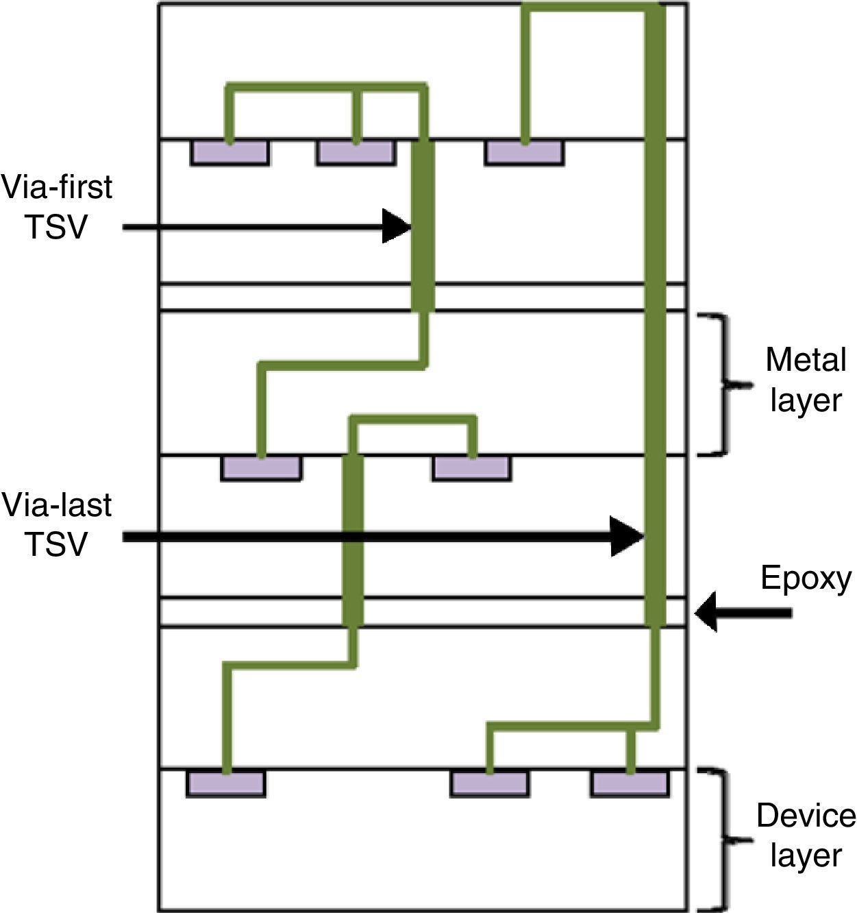
3D-ICs are built up of an IC stack with short vertical interconnections between adjoining dies using through-silicon vias (TSVs). Despite their attractiveness of mitigated congestion and reduced wirelength, TSVs occupy significant silicon area. In addition to increase in die area, excessive use of TSVs will have a negative impact on wirelength in the 3D design (Kim, Mukhopadhyay, & Lim, 2009). There are two types of TSVs: via-first TSVs which reside within the device layer only, and via-last TSVs which occupy both device and metal layers, as illustrated in Fig. 1. Both these types have much larger area footprint than other components (e.g., wires, local vias and gates) (Gerousis, 2010), (Beyne et al., 2008). Therefore, usage of TSVs must be kept minimal in order to exploit their advantages and reduce their negative impact.

Depending on the stacking style, 3D integration is categorized into three types. A basic face-to-face (F2F) type which stacks only two chips face-to-face. For more than two layers, face-to-back (F2B) and back-to-back (B2B) process stacking is inevitable. F2B is the most commonly used multi-chip stacking process hence it is adopted in this paper. Although B2B stacking is also used to stack multiple chips, it requires two TSVs to link two adjacent dies and leads to a larger delay.
In this work, we present a multi-objective circuit partitioning and layer assignment techniques that takes into consideration TSV count minimization and area balancing across all dies. We use simulated annealing (SA) and tabu search (TS) iterative optimization heuristics to achieve these objectives. The rest of this paper is organized as follows. Related work is discussed in Section 2. Section 3 introduces the problem description. Sections 4 and 5 present tabu search and simulated annealing heuristics and their implementation. In Section 6 experimental results are reported and discussed. Finally, Section 7 concludes this work.
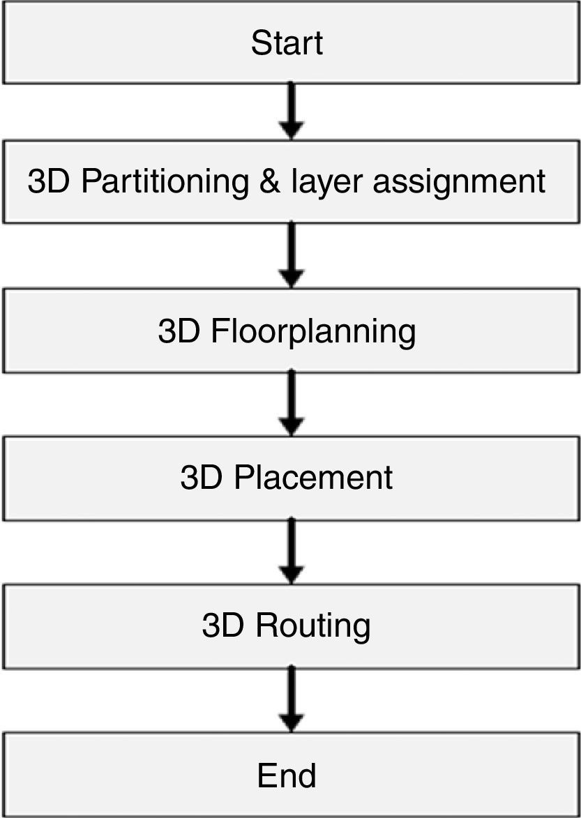
2Related workMuch work has been attempted and discussed in the literature regarding all aspects of the design and implementation of 3D integrated circuits. It has been suggested that it is critical to perform circuit partitioning as an independent stage in the design flow of 3D integration (Chiang & Sinha, 2009; Li et al., 2006; Pavlidis & Friedman, 2009). The flow first partitions a given design into different layers and then solves the remaining problems of floorplanning, placement and routing as shown in Fig. 2. Accordingly, this approach effectively reduces the complexity of the problem and preserves the quality of results (Li et al., 2006; Pavlidis & Friedman, 2009).

Li, Mak, and Wang (2012) proposed computing a tier assignment (i.e., circuit partitioning) based on 1-D placement. They first conduct a traditional 1-D placement of the modules using a spectral method (Hagen & Kahng, 1992). The intuition behind this approach is that tightly connected modules are placed close to each other in the 1-D placement and thus will be assigned to the same layer. The number of TSVs inserted into the ith layer for connecting signals between the ith and the (i+1)th layer is determined by the number of nets crossing the ith cut position. The authors also imposed a constraint on the total area utilized in each layer. Then, they used a dynamic-programming-based algorithm to determine the best L−1 cut positions on the linear placement to obtain an assignment with the minimum number of TSVs while satisfying the area constraint. However, the authors did not take into consideration connections to I/Os in the 1-D placement which will result in additional TSVs in all the layers.
Another approach to solve the partitioning problem employs integer linear programming (ILP) (Lee, Jiang, & Mei, 2012). However, this can only be used for small-size circuits since its runtime grows very fast with problem size. An alternative method is introduced as part of 3D place and route for FPGAs (Ababei, Mogal, & Bazargan, 2006; Siozios, Sotiriadis, Pavlidis, & Soudris, 2007). The authors used a two-step approach. First, they applied the hMetis partitioning algorithm (Karypis, Aggarwal, Kumar, & Shekhar, 1999) to divide a design into a set of partitions. Then, they associated each partition with a layer. A typical partitioning algorithm gives similar weights to cuts between any two partitions, while those weights can have a great impact on the 3D partitioning based on the distance among partitions.
Huang, Liu, and Huang (2011) proposed an iterative layer-aware partitioning algorithm which can minimize the number of TSVs and smooth the distribution of TSVs in 3D structures. The proposed algorithm is iterative and gradually produces the final result layer by layer. The algorithm applies layer-aware partitioning at each iteration. While the focus of the algorithm was on TSV minimization, in this work there was no clear evidence on how the algorithm handled area balancing among layers.
In another work, Kim, Athikulwongse, and Lim (2013) studied the impact of TSVs on various aspects of 3D layouts. These aspects include: maximum allowable TSV count, trade-off between wirelength and TSV count, and wirelength and die area versus number of dies. The authors stated that although they could not draw a clear conclusion on the relationship between wirelength and number of TSVs, using too many TSVs will eventually increase the die area, which will result in wirelength increase.
No non-deterministic algorithms have been attempted to solve the problem of TSV minimization and layer assignment thus far. Therefore, an attempt to use Tabu Search and Simulated Annealing (Sait & Youssef, 1994) is presented in this work. As more design constraints than those reported in the literature are considered, this work can be the base for future work on the partitioning step or the other subsequent steps.
3Problem description3.1MotivationThere are many critical aspects that must be considered when solving the partitioning problem in the context of 3D design flow. These aspects comprise the following points:
- •
Layer assignment: It is a crucial task to be aware of assigning partitions into layers. Usually, different layer assignments result in variance in TSV requirements (Huang et al., 2011).
- •
Location of I/O terminals: all external I/O terminals must be assigned to the top-most layer (or the bottom-most layer). Failing to satisfy this requirement will result in additional TSV requirements in later stages of the design.
- •
TSV minimization: It is desired to have a design with minimal number of TSVs as excessive use of them will increase the area of the design and hence the total wirelength which will eventually degrade the performance of the circuit.
- •
Area balancing: TSVs have a significant area footprint when compared to other components. Thus, an ill-distribution of TSVs across layers will eventually result in a design with imbalanced area. To Achieve this objective, many factors have to be considered, namely, area of cells or blocks, area of TSVs, and distribution of both cells and TSVs across all dies.
Subject to the above requirements, we present in this paper a multi-objective circuit partitioning technique, using iterative non-deterministic heuristics, that takes into consideration: (1) TSV count minimization, and (2) balanced area across all layers or dies.
3.2Problem formulationAny design can be represented as a hypergraph H=(V,E), where V is a set of vertices that include the set of blocks or cells B and the set of I/O terminals I. E is the set of hyperedges that connect vertices from the set V, which in terms corresponds to the netlist of a given design. Therefore, the problem can be mapped into hypergraph partitioning problem to N+1 total partitions P={P0, P1, …, PN}, where the ith layer (partition) belongs to the range 0⩽i⩽N. As all I/O terminals must reside in the top-most layer, all vertices in the set I are assigned to the first partition P0. All other vertices in the set V are assigned to N disjoint partitions {P1, P2, …, PN} such that P1∩P2∩…∩PN=φ. For each vertex v∈V, area(v) denotes the area occupied by v. TSVarea denotes the area cost of a TSV.
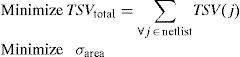
For each net j in the design (i.e., hyperedge e in H) that spans across two layers, we assume that only one TSV is used to connect the subnet in the first layer to the one in the other layer. In general, if net j spans across different layers where u is the upper layer and l is the lower layer, the number of TSVs which is required to connect all subnets of j equals to TSV(j)=u−l. Thus, the total number of required TSVs in the design can be calculated as TSVtotal=∑∀j∈netlistTSV(j).
Given a 3D design and a target N+1 of total partitions, our technique maps the problem into hypergraph H partitioning problem. It partitions the design into N+1 disjoint partitions such that all I/O terminals reside in the first partition (layer) P0. The technique has an objective of minimizing the total number of required TSVs (TSVtotal). It also handles area balancing among the different layers by minimizing the standard deviation of area across all layers, while taking into consideration area of blocks or cells, number of TSVs in each layer, and the area occupied by these TSVs. Thus, it will result in area-balanced TSV-minimized layer-assigned partitions that respect the I/O constraints.
The problem can therefore be formulated as:
Subject to:
4Tabu Search and its implementation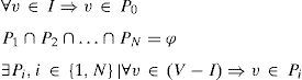
Tabu Search is a general iterative metaheuristic for solving combinatorial optimization problems. TS progresses by making iterative perturbations while preventing cycling to certain number of recently visited points in the search space. TS procedure starts from an initial feasible solution S (current solution) in the search space Ω. A neighborhood ℵ(S) is defined for each S. A sample of neighbor solutions V*⊂ℵ(S) is generated called trial solutions (n=V*≪ℵ(S)), and comprises what is known as the candidate list. From this generated set of trial solutions, the best solution, say S*∈V∗ is chosen for consideration as the next solution. A solution S*∈ℵ(S) can be reached from S by an operation called a move to S*. The move to S* is considered even if S* is worse than S, that is, Cost(S*)>Cost(S). Selecting the best move in V* is based on the supposition that good moves are more likely to reach the optimal or near-optimal solutions. The best candidate solution S*∈V∗may or may not improve the current solution, but is still considered. It is this feature that enables escaping from local optima. However, with this strategy, it is possible to reach the local optimum, since moves with Cost(S*)>Cost(S) are accepted, and then in a later iteration return back to local optimum.
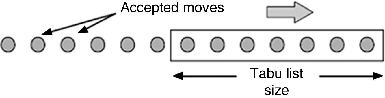
In order to block returning to previously visited solutions a memory or list T, known as tabu list, is maintained. This list contains information that to some extent forbids the search from returning to a previously visited solution. Whenever a move is accepted, its attributes are introduced into the tabu list T. Move reversal are prevented for next k=|T| iterations because they might lead back to a previously visited solution. The tabu list can be visualized as a window on accepted moves as shown in Fig. 3; moves which tend to undo previous moves within this window are forbidden.

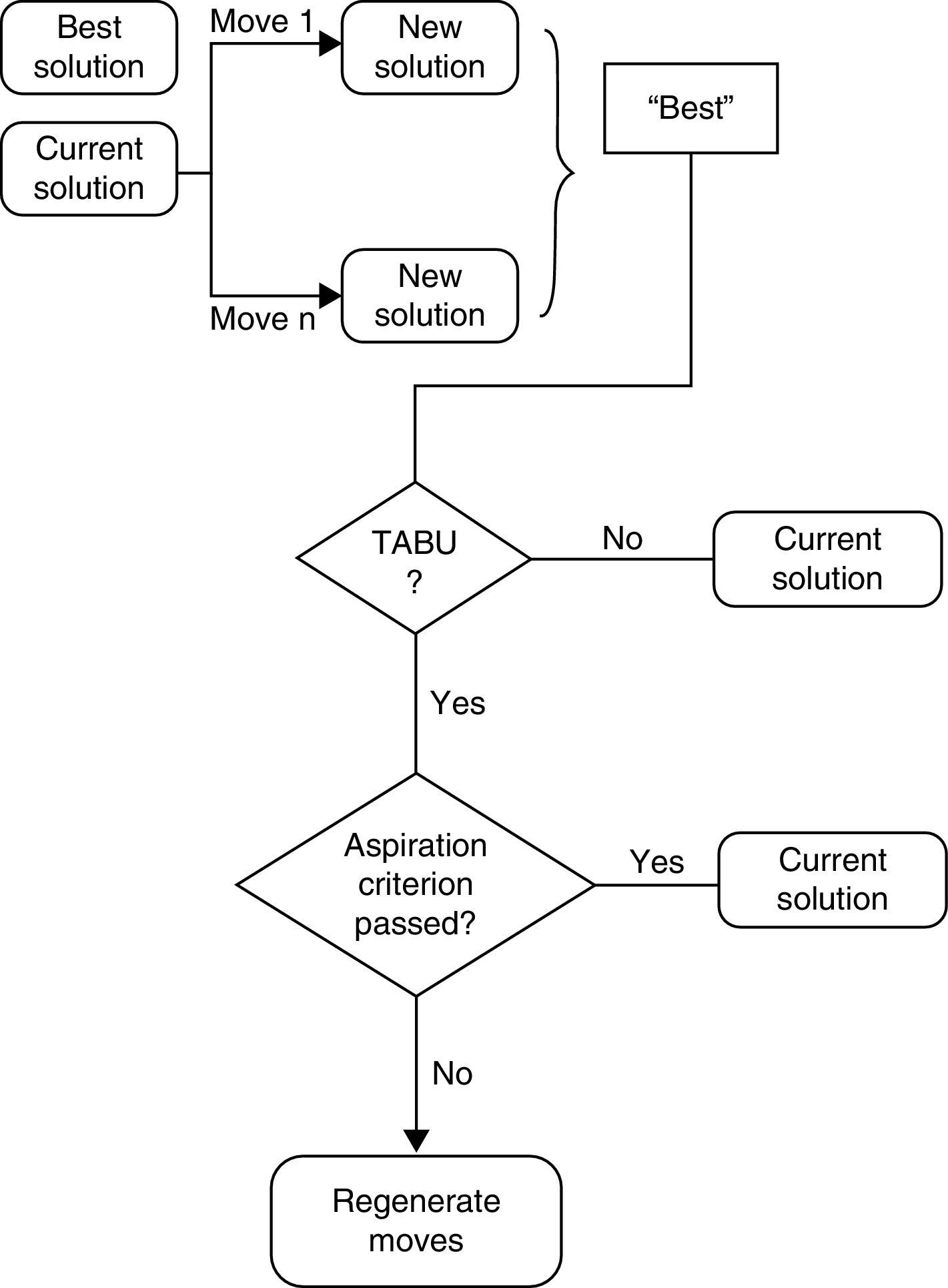
In some cases, it is necessary to overrule the tabu status since only move attributes (not complete solutions) are stored in tabu lists. These tabu moves may also prevent the consideration of some solutions which were not visited earlier. This is done with help of the notion of aspiration criterion. Aspiration criterion is a device used to override the tabu status of moves whenever appropriate. Aspiration criterion must make sure that the reverse of a recently made move leads the search to an unvisited solution, generally a better one (Sait & Youssef, 1999). A flow chart illustrating the basic short-term memory tabu search algorithm is given in Fig. 4. Intermediate-term and long-term memory processes are used to intensify and diversify the search respectively (Sait & Youssef, 1999).

One of the Tabu Search algorithm parameters is the size of the tabu list. A small tabu list size is preferred for exploring the solution near a local optimum, and a larger tabu list size is preferable for breaking free of the vicinity of local minimum. List sizes varying between 5 and 12 have been used in many applications (Sait & Youssef, 1999). Any aspect (feature or component of a solution) that changes as a result of a move from S to Strial can be an attribute of that move. A single move can have several attributes. The duration for which a move containing the particular tabu attribute is forbidden (the size of tabu list) is called Tabu tenure. An algorithmic description of a simple implementation of the tabu search is given in Fig. 5.
4.1Solution representation and initialization.")
Since the problem is mapped into a graph partitioning and layer assignment, the solution is represented as a number of partitions each of which corresponds to a layer in the 3D structure. The first partition, which represents the top-most layer, includes all the I/O terminals. Other blocks or cells of the circuit are assigned to one of the other partitions. In the initialization step, all I/O terminals are assigned to the first partition, while blocks are randomly assigned to the remaining partitions.
4.2Cost evaluationThe cost function is a measure of how good a particular solution is. For 3D partitioning and assignment, there are two main criteria: area balancing and TSV count. The cost function should reflect all objectives. Traditionally, multi-objective problems are implemented by combining the objectives into a scalar function like the weighted sum of the multiple attributes. Usually, it is difficult to determine suitable weights for these objectives as their values belong to different ranges.
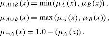
One practice is to use fuzzy logic to handle these types of multi-objective problems (Sait & Youssef, 1999; Zadeh, 1965; Zadeh, 1973; Zadeh, 1975). Unlike ordinary set theory where an element is either in a set or not, in fuzzy set theory, an element partially belongs to a set with a certain degree of membership. This is realized by using a membership function μA(.) that maps the space of points (solutions) to the interval [0,1]. Operations like union (∪), intersection (∩), and complementation (¬) which are used in ordinary set theory have been defined for operations on fuzzy sets. One such logic is defined by Zadeh and called the min-max logic (Sait & Youssef, 1994). In this logic, the above operations are defined as follows:
The evaluation of a solution comprises the evaluation of fuzzy rules which return a value that corresponds to the degree of membership of that solution in the fuzzy subset of good solutions. The fuzzy logic rules are usually expressed on problem-specific linguistic variables (Zadeh, 1965; Zadeh, 1973; Zadeh, 1975).
In our case, the objective is to find a solution which is optimized with respect to TSV count and the standard deviation in area across all partitions. To obtain a fuzzy logic definition of the above multi-criteria objective function, two linguistic variables, tsv-count and area-deviation, are introduced and a linguistic value “low” and “small” for each of them, respectively, is defined. These linguistic values characterize the degree of satisfaction of the designer with the values of objectives.
Membership functions for low tsv-count μtsv and small area-deviation μarea are built easily. These are non-increasing functions, since the lower the tsv-count and smaller the area-deviation, the higher is the degree of satisfaction. The base variables tsv-count and area-deviation are normalized to the interval [0,1] as shown in Fig. 6. The values Tmin and Dmin are lower bounds on the TSV count and area deviation. Tmin equals to the number of nets that have an I/O terminal. This is based on the assumption that all blocks which belong to these nets are assigned to the layer next to the I/O layer; one TSV is used to connect the I/O terminal to its associated net in the next layer. Dmin equals to 0, assuming that the sum of areas of blocks and areas of TSVs in all layers is the same. The values of Tmax and Dmax are corresponding to the upper bounds. Tmax equals to the number of nets multiplied by number of layers (# nets×(# layers – 1)). In theory, it has been proven that the upper bound of the standard deviation of a set of data with three or more elements can not exceed 58% of the range of that set (Croucher, 2002; Croucher, 2004; Lee, Lee, & Lee, 2006). Therefore, the value of Dmax is set to 58% of the range between maximum and minimum area.

The most desirable solution is the one with the highest membership in the fuzzy subsets low tsv-count and small area-deviation. However, such a solution most likely does not exist. Therefore, one has to trade-off these individual criteria with each other. A weighted averaging operator (Fodor & Roubens, 1994; Fodor & Roubens, 1992; Fodor, Marichal, & Roubens, 1995) is used to incorporate this trade-off as follows:
where μS is the membership function of the fuzzy subset of good solutions, and β is a parameter between 0 and 1. When β=1, the focus becomes on the tsv-count objective, and for β=0 the focus is switched to the other objective.4.3Neighborhood solutions generation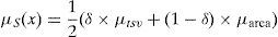
TS makes several neighborhood moves and selects the move producing the best solution among all candidate moves for current iteration. This best candidate solution may not improve the current solution. In each iteration, a number of neighbor solutions (i.e., equal in number to the size of the candidate list) are generated by making perturbations as follows:
- (1)
75% of the time two random blocks will be selected from two random layers, and their respective layers interchanged.
- (2)
25% of the time one random block will be selected from a random layer, and it will be moved to another randomly selected layer.
Subsequently, each solution in the candidate list is evaluated using the fuzzy function in Eq. (1) based on the change in number of TSVs and the standard deviation of area among different layers before and after the swap/move. If two or more neighborhood solutions have equal swap cost, one of them will be selected.
4.4Tabu list and aspiration levelVariety of tabu attributes were tested, when blocks (cells) are swapped/moved. One experiment considered both i and j, forbidding any perturbations that include both of them. Another attribute was to forbid moves related to block i, i.e., any move which include i, this covers the reverse of swapping i with j. The second attribute of a move is used in all results reported in this paper. If two blocks are involved in interchange, any move that includes any of these two blocks is forbidden. The same applies for moving blocks from one layer to the other. A short-term memory element is used throughout the implementation where tabu list sizes ranging from 5 to 12 were tested. The change in tabu list size in this range has little impact on the quality of the solutions; therefore the size of tabu list was set to 10. The aspiration criterion is implemented as follows: tabu restriction is overridden if the current solution is the best seen so far, and the current solution is accepted as new best solution and tabu list is updated. In the next section, simulated annealing iterative heuristic is discussed. Details about the parameters used in this work are reported in Section 4.
5Simulated annealing and its implementationSimulated annealing is a general heuristic and one of the most well developed iterative techniques. It is widely used for solving optimization problems. One important feature of simulated annealing is that, like tabu search, it also accepts solution with deteriorated cost. It is this feature that gives the heuristic the hill climbing capability. Initially, the probability of accepting inferior solutions is large; but as the search progresses, only smaller deteriorations are accepted, until finally only good solutions are accepted. In order to simulate the annealing process, much flexibility is allowed in neighborhood generation at higher “temperatures”, i.e., many ‘uphill’ moves are permitted at higher temperatures. The temperature parameter is lowered gradually as the search progresses. As the temperature is lowered, fewer and fewer uphill moves are accepted. In fact, at absolute zero, the simulated annealing algorithm turns greedy, allowing only downhill moves.
The iterative improvement scheme starts with some given state, and examines a local neighborhood of the state for better solutions. A local neighborhood of a state S, denoted by ℵ(S), is the set of all states which can be reached from S by making a small change to S.
The simulated annealing algorithm is shown in Fig. 7. The core of the algorithm is the Metropolis procedure, which simulates the annealing process at a given temperature T (Fig. 8) (Metropolis, Rosenbluth & Teller, 1953). The Metropolis procedure receives as input the current temperature T, and the current solution CurS which it improves through local search. Finally, Metropolis must also be provided with the value M, which is the amount of time for which annealing must be applied at temperature T. The procedure Simulated_annealing simply invokes Metropolis at decreasing temperatures. Temperature is initialized to a value T0 at the beginning of the procedure, and is reduced in a controlled manner (typically in a geometric progression); the parameter α is used to achieve this cooling. The amount of time spent in annealing at a temperature is gradually increased as temperature is lowered. This is done using the parameter β>1. The variable Time keeps track of the time being expended in each call to the Metropolis. The annealing procedure halts when Time exceeds the allowed time (Sait & Youssef, 1999).


The Metropolis procedure is shown in Fig. 8. It uses the procedure Neighbor to generate a local neighbor NewS of any given solution S. The function Cost returns the cost of a given solution S. If the cost of the new solution NewS is better than the cost of the current solution CurS, then the new solution is accepted, and we do so by setting CurS=NewS. If the cost of the new solution is better than the best solution (BestS) seen thus far, then we also replace BestS by NewS. If the new solution has a higher cost in comparison to the original solution CurS, Metropolis will accept the new solution on a probabilistic basis. A random number is generated in the range 0 to 1. If this random number is smaller than e−ΔCost/T, where ΔCost is the difference in costs, (ΔCost=Cost(NewS)−Cost(CurS)), and T is the current temperature, the uphill solution is accepted. This criterion for accepting the new solution is known as the Metropolis criterion. The Metropolis procedure generates and examines M solutions.
The probability that an inferior solution is accepted by the Metropolis is given by P(RANDOM<e−ΔCost/T). The random number generation is assumed to follow a uniform distribution. Remember that ΔCost>0 since we have assumed that NewS is uphill from CurS. At very high temperatures, (when T→∞), e−ΔCost/T≃1, and hence the above probability approaches 1. On the contrary, when T→0, the probability e−ΔCost/T falls to 0.
In order to implement simulated annealing, the same cost function formulated in Section IV is used. In addition, similar techniques are used to implement the Neighbor function to generate new states from current states.
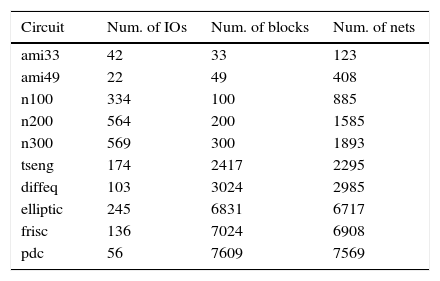
6Experimental resultsThe algorithms described in this work were implemented and tested on a set of benchmark circuits to solve the L-way partitioning and assignment problem, where L is the number of layers. These include small, medium, and large size circuits (“MCNC/GSRC benchmarks,” n.d.; Yang, 1991). Table 1 reports these circuits and their respective number of IOs, blocks, and nets.
After many experiments and fine tuning to the parameters of the iterative heuristics, a candidate list of size 25 is used for tabu search; the tabu list size is set to 10. For simulated annealing, different values for parameters α, β, and M were tested and the value of α=0.98, β=1.001, and M=50 were found suitable. The initial temperature, T0, was determined using the classical heating method by experiment with increasing temperatures until the probability of accepting of both good and bad moves was very high. Simulation was by setting the temperature to 1, and then increasing until 100. Acceptable values of T0 were found to be in the range [40,50]. The number of iterations for TS is fixed to 4,000. Since the candidate list size in TS is 25, for the sake of comparison simulated annealing is allowed to run for 4000×25=100,000 iterations. The objective is set to partition the design into 4 layers in addition to the I/O layer. The total number of TSVs reported later includes TSVs that connect I/O terminals to other blocks in the circuit. The size of a TSV, TSVarea, is fixed to 10 units. The value of the weight of the total membership function δ is set to 0.8 in Eq. (1).
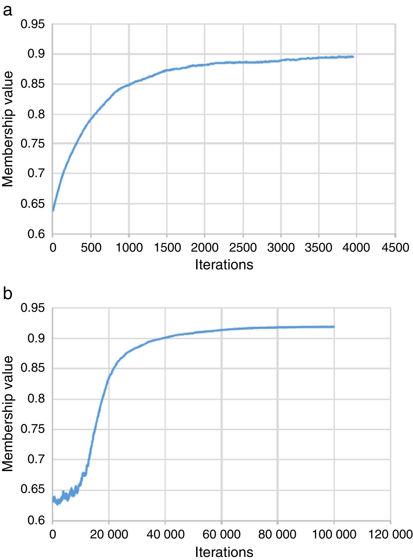
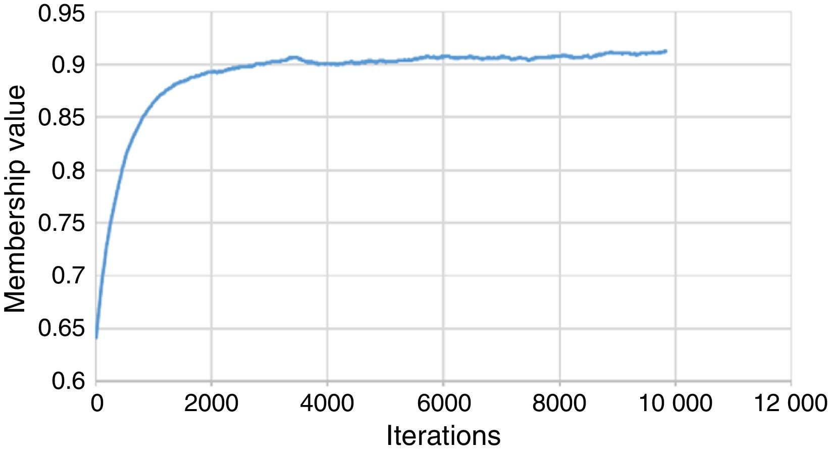
The performance of the presented algorithms is compared considering different aspects. Fig. 9 shows a plot of the values retrieved by the fuzzy cost function, that is membership value of the solution, versus the number of iterations for the “tseng” circuit for both TS and SA. Recall that the TS and SA are seeking to maximize the membership function. In this regard, SA outperformed TS as it achieved a higher membership value. After a little bit of almost a random behavior where the initial temperature is high, simulated annealing sharply achieved an improvement from 0.65 up to 0.85. Later on, it went up on a slower pace until it almost saturated around a membership value of 0.92. On the other hand, TS showed a steady improvement which started sharply at the beginning and then continued slow and steady. TS could not pass the 0.9 threshold in the given time. However, giving TS enough time should eventually lead to better solutions as TS can always escape local minima. To verify this, Fig. 10 shows the performance of tabu search when the run-time is extended to 10,000 iterations and the candidate list size is increased to 40. It is evident that, given enough run-time, tabu search can produce high quality solutions.
 tabu search; (b) simulated annealing.")

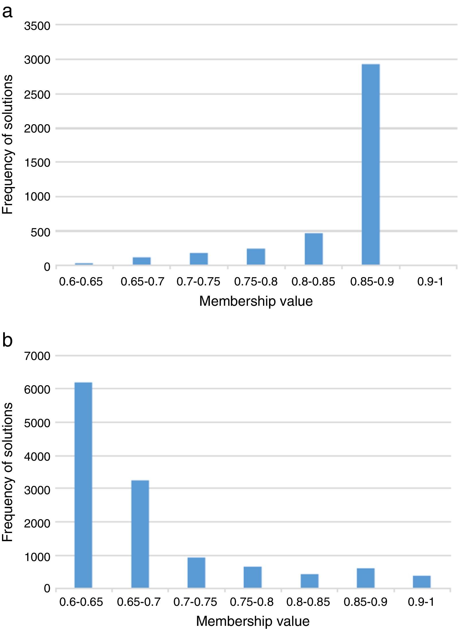
Another experiment consists of comparing the two heuristics with respect to the searched spaces. Results are summarized in Fig. 11 in the form of bar charts. TS exhibited the best performance, while SA was behind. This figure depicts where each algorithm spent its time. TS concentrated its efforts in good subspaces, i.e., evaluating solutions with high membership values. In contrast, SA spent most of its time evaluating poor quality solutions as it starts with almost a random behavior at the initial temperature. These behaviors were observed with all test cases. Tabu search showed a better behavior in general. As shown earlier in Fig. 10, giving enough time, it can produce high quality results. Thus, the termination criterion, i.e., number of maximum iterations, can be decided later based on the application and the time constraint.
 tabu search; (b) simulated annealing.")
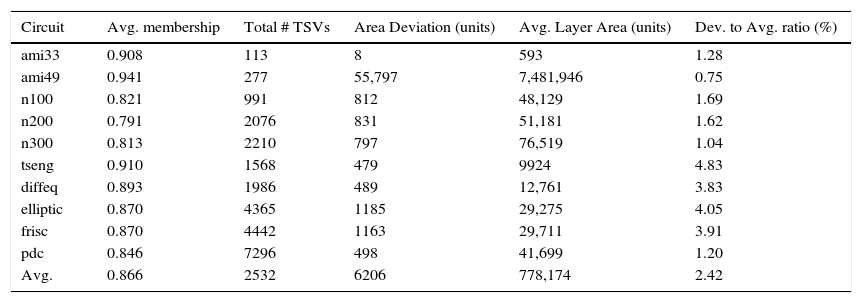
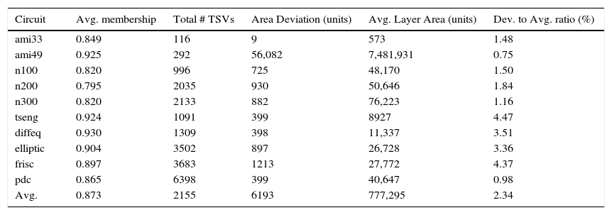
Finally, Tables 2 and 3 report detailed results about the application of TS and SA respectively. In these tables membership values of the fuzzy cost function, total number of the required TSVs, standard deviation of area across all layers (in units), average layer area, and the percentage of area deviation to the average area are presented (average values of different runs are reported in these tables). Both algorithms exhibited a good performance on small as well as large circuits. It is evident that, in terms of membership value of the fuzzy cost function, SA has achieved better results when compared to TS in most of the cases in our setup. This membership value translates itself to the total number of required TSVs and the standard deviation in area across different layers. A higher membership value could result in a better TSV count and a better area deviation, or at least one of them. If we look at the “n100” circuit in the two tables, we observe almost the same membership value. However, in the first table, associated with TS, it results in a better TSV count and a worse area deviation as compared to the second table which is associated with SA. In the used setup, SA outperformed TS in achieving a better TSV count and area deviation especially for large circuits like “tseng”, “diffeq”, “elliptic”, and “pdc”. The standard deviation of area for all the cases is less than 5% with an average around 2.4%. Unfortunately, we could not compare our results with the ones reported in (Huang et al., 2011) as they did not report the area deviation. Moreover, number of TSVs reported for some circuits is less than number of nets with I/O connections which contradicts with both our assumptions and practicality. For example, “aqua” circuit has 3792 IOs and the reported number of required TSVs for this circuit is 909.6 (Huang et al., 2011). However, the results presented in this work can be the base for future work on the partitioning step or the other subsequent steps.
Tabu search results with: 4,000 iterations, candidate list size=25, and tabu list size=10.
| Circuit | Avg. membership | Total # TSVs | Area Deviation (units) | Avg. Layer Area (units) | Dev. to Avg. ratio (%) |
|---|---|---|---|---|---|
| ami33 | 0.908 | 113 | 8 | 593 | 1.28 |
| ami49 | 0.941 | 277 | 55,797 | 7,481,946 | 0.75 |
| n100 | 0.821 | 991 | 812 | 48,129 | 1.69 |
| n200 | 0.791 | 2076 | 831 | 51,181 | 1.62 |
| n300 | 0.813 | 2210 | 797 | 76,519 | 1.04 |
| tseng | 0.910 | 1568 | 479 | 9924 | 4.83 |
| diffeq | 0.893 | 1986 | 489 | 12,761 | 3.83 |
| elliptic | 0.870 | 4365 | 1185 | 29,275 | 4.05 |
| frisc | 0.870 | 4442 | 1163 | 29,711 | 3.91 |
| pdc | 0.846 | 7296 | 498 | 41,699 | 1.20 |
| Avg. | 0.866 | 2532 | 6206 | 778,174 | 2.42 |
Simulated annealing results with: 100,000 iterations, α=0.98, β=1.001, M=50, and the initial temperature, T0, in the range [40,50].
| Circuit | Avg. membership | Total # TSVs | Area Deviation (units) | Avg. Layer Area (units) | Dev. to Avg. ratio (%) |
|---|---|---|---|---|---|
| ami33 | 0.849 | 116 | 9 | 573 | 1.48 |
| ami49 | 0.925 | 292 | 56,082 | 7,481,931 | 0.75 |
| n100 | 0.820 | 996 | 725 | 48,170 | 1.50 |
| n200 | 0.795 | 2035 | 930 | 50,646 | 1.84 |
| n300 | 0.820 | 2133 | 882 | 76,223 | 1.16 |
| tseng | 0.924 | 1091 | 399 | 8927 | 4.47 |
| diffeq | 0.930 | 1309 | 398 | 11,337 | 3.51 |
| elliptic | 0.904 | 3502 | 897 | 26,728 | 3.36 |
| frisc | 0.897 | 3683 | 1213 | 27,772 | 4.37 |
| pdc | 0.865 | 6398 | 399 | 40,647 | 0.98 |
| Avg. | 0.873 | 2155 | 6193 | 777,295 | 2.34 |
In this work we provided a multi-objective circuit partitioning and layer assignment techniques, using iterative optimization heuristics namely Tabu Search and Simulated Annealing, that takes into consideration TSV count minimization, and area balancing across all layers while including the I/O constraint. Both the heuristics have been engineered to tackle this problem. They both were able to produce a high quality outcome. The average percentage of the area deviation compared to the average area of a layer was around 2.4% in addition to minimizing the total number of required TSVs.
Conflict of interestThe authors have no conflicts of interest to declare.
Authors acknowledge King Fahd University of Petroleum & Minerals for all support.
Peer Review under the responsibility of Universidad Nacional Autónoma de México.