


In this paper we show the importance of applying mathematical optimization when designing the distribution network in a supply chain, specifically in making decisions related location of facilities and inventory management, which are associated with different levels of planning but are closely related.
The addressed problem is an extension of the classic capacitated facility location problem. The distinguishing features are: the inventory management, the presence of multiple plants, and the single source constraints in both echelons. A key issue is that demand at each distribution center is a function of the demands at the retailers assigned, which is a random variable whose value is not known at the time of designing the network. We focus on the mathematical modeling of the problem and the evaluation of the performance of the developed models, so, it can be observed the troubles that arise when modeling supply chains that consider different types of decisions.
En este artículo se muestra la importancia de la optimización matemática en el diseño de una cadena de suministros, especificamente en la tóma de decisiones dentro de un problema de localización de instalaciones y un problema de inventarios. Dichas decisiones pertenecen a diferentes niveles de planeación aun así se encuentran estrechamente relacionadas.
El problema es una extensión del clásico problema de localización de instalaciones capacitadas. Las características destacadas son: el manejo de inventarios, la presencia de múltiples plantas y las restricciones de única fuente en ambos niveles de la cadena. Un punto clave en la investigación consiste en definir la demanda de los centros de distribución como función de la demanda de los minoristas asignados, la cual es una variable aleatoria, cuyo valor es desconocido al momento de diseñar la red de distribución. Nos enfocamos en la modelación matemática del problema y en la evaluación del desempeño de los modelos desarrollados, de manera que es posible observar la dificultad que involucra modelar cadenas de suministros que consideran diferentes tipos de decisiones.
In a highly competitive world, companies must ensure an efficient use of resources. For this purpose, supply chain management must focus on an efficient integration of productive actors. This topic has been subject of intense research and several types of approaches can be used. See, for example, the survey presented by Pires et al. [1] about resource selection (productive actors).
Other important consideration in the supply chain management is the interaction between tactical, operational and strategic decisions. References [2,3,4] show an overview of this trend.
We address in this work the design of a twoechelon distribution network for a supply chain through a joint location inventory problem. Location decisions are typically classified as strategic decisions and their importance is obvious because they involve large monetary investments and long periods of time. On the other hand, inventory decisions belong to the operational level and their impact is not so obvious. However, its influence on the supply chain has been increasingly recognized in the last years and philosophies like just in time or lean manufacturing consider the reduction of stock as a basic principle.
Among some publications involving location and inventory problems we can mention the work of Tancrez [5], which incorporates the Economic Order Quantity Model (EOQ) into the facility location problem, assuming deterministic demand and fixing the lot size. References [4,6,7,8] present similar problems, but assume stochastic demands. Hernández et al. [9] develop an algorithm to solve multi item inventory decisions.
Usually, a mixed integer nonlinear program (MINLP) is formulated when modeling problems that involve inventory costs, although there are some papers that use some linear approximations [9, 10, 11].
Regarding to solution methods, the literature is not very extensive. The Lagrangian relaxation is the most appealed tool for solving problems with similar characteristics [8], but heuristics have also been used [7,10].
The most distinctive feature in the problem tackled in this paper is the consideration of multiple plants. Having alternatives when choosing plants, involves the presence of allocation decisions, which in our case are single source constraints. This means that each demand point should be serviced by a single supply point. Some papers involve several choices for plants, but they model under the assumption that the values of the parameters corresponding to these plants, i.e., delivery time and shipping cost are the same regardless of which distribution centers they serve. With this assumption, it does not matter which plant serves each distribution center, thus eliminating allocation decisions and therefore, greatly simplifying the problem.
This article focuses on the mathematical modeling of the problem and is organized as follows. The second section presents the formal description of problem, assumptions and features to meet the supply chain. The third section is dedicated to our mathematical formulation, explaining the three developed models: a mixed integer nonlinear programming model, a mixed integer linear programming model and a binary integer linear programming model. Models'; evaluation and sensitivity analysis applied to the selected model is shown in computational results section. Finally, conclusions and future work are presented in the fifth section.
2Problem descriptionThe problem arises in a network of a supply chain consisting of plants, distribution centers (DC) and retailers. We assume each retailer has uncertain demand of a single product with normal distribution. We want to find the network configuration that meet retailer demands, at a minimum cost, without violating capacity and single-source constraint.
The total cost includes fixed costs for opening distribution centers, costs associated with transportation through the chain and inventory costs in the opened facilities. The decisions are: determine the appropriate number of distribution centers that should be opened and their location, the assignment of distribution centers to plants and assignment of retailers to distribution centers. The assignment must be done in such a way that every open distribution center is attended by a single plant, likewise, each retailer must be served just by a single open distribution center.
Location of plants and customers (retailers) is known, as well the production capacity of the plants. Customer demand behaves following a normal distribution with estimated mean and variance. Concerning to the demand of distribution centers, this is a function of retail demand, taking advantage of the phenomenon known as “risk pooling” and avoiding the “bullwhip effect”. This idea is based on the assumption for sharing the risks of demand's variability, as the increase in demand of a customer is balanced with the decrease in demand for another client.
Holding costs are the same for all distribution centers. Working inventory and safety stock will be considered only in the distribution centers, which will follow the Economic Order Quantity Model [13].
Shipping costs from plants to distribution centers consider economies of scale and therefore are modeled through a fixed cost and a variable cost. Unsatisfied demand is controlled by setting a desired service level, which is measured as the probability that distribution centers will be stocked during the delivery times. These features have been included inspired on real world problems in supply chains.
3Model FormulationThe following notation will be used throughout this paper.
3.1SetsK: Set of retailers, indexed by k. Set of candidate distribution centers sites, indexed by j. Set of plants, indexed by i.
dk Mean of daily demand for each retailer k. Number of working days in a year. Variance of the daily demand for each retailer k. Fixed annual cost for locating a distribution center at site j. Weight factor associated with the shipment cost. Weight factor associated with the inventory cost. Annual holding cost per ítem. Fixed cost for placing an order from distribution center j. Lead time in days for deliveries from plant to distribution center j. Variable cost of shipping an order from plant i to distribution center j. Unit shipment cost from plant to distribution center j. Unit shipment cost from distribution center j to retailer k. Probability of meeting the demand during lead time. Production capacity of plant Capacity of distribution center Value of the standard normal distribution, which accumulates a probability of ¿. Auxiliary parameter whose value is equal to ¿¿hz¿
Let us introduce the following variables, which will be used in the first model.
3.3.1Decision variablesXj = 1, if j is selected as a distribution center location, and 0 otherwise; for each j ∈ J.
Yjk = i, if the retailer k is served by a distribution center located at j, and 0 otherwise; for each j ∈ J and each k ∈ K.
Zij = 1, if distribution center located at j is served by a plant i and 0 otherwise; for each j ∈ J and each i ∈ I.
3.3.2Auxiliary variables related to distribution centersSj Variance of the daily demand for each distribution center j. Mean of daily demand for each distribution center j. Lead time in days for deliveries at each distribution center j.
Now, our first model is formulated as follows:
s.t: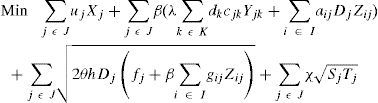


The objective function minimizes the total weighted cost of the distribution network. The first term in (1) calculates the cost for locating distribution centers, while the costs for transporting products from plants to distribution centers and shipping costs of products from DCs to customers are simplified in the second term. The weighted cost for holding inventory, ordering cost and variable cost to send orders to the selected centers are shown simplified in the third term of (1). The last sum corresponds to the weighted cost for holding safety stock.
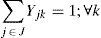
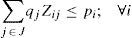
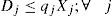
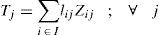
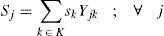
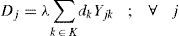
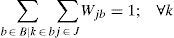
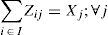
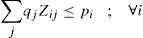
Regarding to constraints, equation (2) ensures that each retailer is assigned to a single DC, while (3) ensures that each open center is assigned to a single plant. Inequalities (4) and (5) are capacity constraints for plants and DCs respectively. Expression (6) defines the lead time from distribution centers to retailers. Constraint (7) expresses the variance of the daily demand for each distribution center. Constraint (8) defines the average annual demand for each distribution center; this demand is the sum of individual demands of the retailers assigned to each DC.
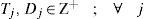
Finally (9)–(11) establish the nature of the variables. This model is a mixed integer nonlinear programming model; we will refer to it later as MINLP.
As will be seen subsequently, it was not possible to find optimal solutions using this model, even after pre-processing and trying several solvers. For this reason, we decided to look for a new formulation.
3.4Mixed integer linear programming modelIt is not difficult to see that the problem could be visualized in another way. Specifically, a subset of retailers could be pre-assigned to a distribution center enable to meet its demand, and then assign the selected center to a plant, minimizing cost at the same time. With this idea in mind, consider additionally the following set and variables which are necessary to establish the new formulation.
3.4.1SetB: Set of all possible subsets b of the retailers set, that is the power set of K without considering the empty set.
Obij = 1, if plant i serves distribution center j which serves the set of retailers b, 0 otherwise; for each b ∈ B, i ∈ I and j ∈ J.
Wjb = 1, if distribution center j serves the set of retailers b, 0 otherwise; for each, b ∈ B, j ∈ J.
The resulting model is a mixed integer linear model (hereinafter referred to as MILP). It is expressed as follows:
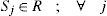
s.t:Where Mbij represents the cost for ordering, holding inventory and transportation regarding plant i, distribution center j and subset of retailers b. Note that nonlinear terms remain, however, now they only involve parameters, variables are no longer involved. It is expressed mathematically as follows:The first term of the objective function (12) remains as before, it represents the cost for opening distribution centers, while the latter corresponds to shipping costs between distribution centers and retailers.
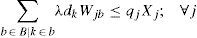


Constraint (13) assures that each retailer is assigned to a single subset and served exactly by a single distribution center. The expression (14) states that opened distribution centers must be assigned to single plants. Constraints (15) and (16) avoid exceeding the capacity of plants and DC, respectively.
Variables Obij act as indicators of arcs activation between the two levels of the chain. See constraint (17), which relates links between plants and distribution centers (Zij = 1) and links related to distribution centers and retailers. Finally, constraints (18) state the nature of the decision variables.
It is important to emphasize that MILP and MINLP have the same search space; all the possible assignments are the same in both cases. Considering the set of all possible subsets of retailers in MILP, it is possible to calculate the inventory and transportation costs before optimizing and the new model turned out to be linear.
The disadvantage of this model is that the number of constraints and variables grows exponentially. To lessen a bit the size of the set B, we decided to eliminate in advance, those sets with demand greater than the capacity of the largest distribution center, as they violate constraint (15). Even so, accurately resolution was only possible for small instances, that is, sets with few elements. For that reason, we tried a reformulation, described next, that allows solving larger instances.
3.5Reformulating MILP as a binary integer linear programming model.For this formulation, we consider subsets of retailers that can be served by the distribution centers and decide in advance the assignment to each of them. Obviously, a subset of retailers is assigned to a specific distribution center only if its demand is less than or equal to the capacity of that distribution center.
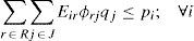
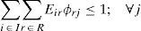
Then, we introduce a new element: “star”. This element is a subset of retailers, which is assigned to a distribution center with enough capacity to support joint demand that integrates retailers. We denote this set by r and the set of all possible assignments retailers-distribution center by R. Thus, the decisions that should be made are to choose stars and assign them to a plant. We need the following variable:
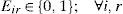
Eir = 1, if plant i serves star r, and 0, otherwise; for each i ∈ I and r ∈ R.
The cost of the plant-star assignment is a function of the plant and the elements involved in the star, thus becoming a parameter so the objective function becomes linear. The resulting model is a binary integer linear programming model; we refer to it as BLP.
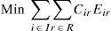

Where
R:Set of stars indexed by r.
¿kr: Binary matrix, where each component takes the value 1 if retailer k belongs to star r; 0 otherwise.
¿jr: Binary matrix, where each component takes the value 1 if distribution center j belongs to star r; 0 otherwise.
Cir: Total cost generated by assigning star r to plant i. It includes the cost for opening the DC, inventory cost and transportation cost.
Recalling constraint (5) and constraint (15) in MINLP and MILP respectively, the demand of the retailers assigned to a distribution center should respect its capacity, which mean that a set of retailers is never assigned to a distribution center without enough capacity to supply them. In BLP, this condition is already established at the time that stars are defined. This shows that BLP only discards infeasible solutions before optimizing, but it has the same search space than previous models and therefore the models are equivalent. Moreover, as we will discuss in the next section, this model handles fewer elements than the previous ones, streamlining the optimization time and allowing solve larger instances.4Computational results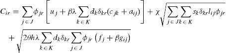
In this section we show the results obtained from computational experiments. We performed two sets of experiments, the first one focused on evaluating the formulations in order to choose the best. The evaluation criteria were: runtime, optimality scope and size of solved instances. The second set of experiments was conducted using the best model, performing a sensitivity analysis on the network configuration parameters (service level and weight factor associated with shipment and inventory).
4.1Models evaluationWe generated eight instances and solved them using GAMS 22.8, a mathematical programming and optimization software interface with various optimization libraries. The instances were solved on a sun Fire V440 processor, connected to 4 of 1602Hhz Ultra Sparc III with 1MB cache and 8GB memory.
We used AlphaECP v1.63, a solver based on the extended cutting plane method, to solve the first model (MINLP) and CPLEX v11.1.1 was used for the other two.
The instances are determined by the number of plants, DC and retailers varying in the following way:
Plants: 2≤|I|≤6
Distribution Centers: 3≤|J|≤7
Retailers: 4≤|K|≤12
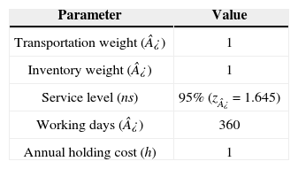
The parameters were determined trying to follow real life situations, others were chosen by keeping feasibility of the model. Table 1 presents some of the parameters used in this experiment.
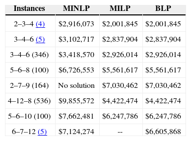
Table 2 highlights the results obtained when solving the instances with each model. First column indicates the size of the instance: the three first numbers represent the number of plants, potential distribution centers and retailers, respectively. The number in parentheses is the seed used to generate the random parameters. The value of the objective function is shown in the next three columns for each model; it is expressed in monetary units.
Best objective values found by each model.
| Instances | MINLP | MILP | BLP |
|---|---|---|---|
| 2–3–4 (4) | $2,916,073 | $2,001,845 | $2,001,845 |
| 3–4–6 (5) | $3,102,717 | $2,837,904 | $2,837,904 |
| 3–4–6 (346) | $3,418,570 | $2,926,014 | $2,926,014 |
| 5–6–8 (100) | $6,726,553 | $5,561,617 | $5,561,617 |
| 2–7–9 (164) | No solution | $7,030,462 | $7,030,462 |
| 4–12–8 (536) | $9,855,572 | $4,422,474 | $4,422,474 |
| 5–6–10 (100) | $7,662,481 | $6,247,786 | $6,247,786 |
| 6–7–12 (5) | $7,124,274 | -- | $6,605,868 |
As can be observed, no optimal solutions could be found with MINLP model, the values of the objective function are greater than the ones found with the others models. The gap between solutions obtained by MINLP model and solutions obtained by linear models reaches 30% in some cases. In addition MINLP could not find even a feasible solution for one instance. On the other hand, MILP and BLP models reach optimal values, but only BLP model is able to solve all test instances. Recall that the set of retailers produces an exponential growth in the number of variables and constraints, so MILP model becomes computationally intractable for more than 10 retailers.
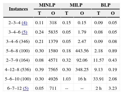
Table 3 summarizes the computation time required for each model. It specifies two times, the first one titled as “T” refers to the time required for preprocessing, compiling and executing the model, while the second one (“O”) is the optimization time required by the optimizer to solve the case. Time is measured in seconds, unless otherwise is indicated.
Time required for solving the instances.
| Instances | MINLP | MILP | BLP | |||
|---|---|---|---|---|---|---|
| T | O | T | O | T | O | |
| 2–3–4 (4) | 0.11 | 318 | 0.15 | 0.15 | 0.09 | 0.05 |
| 3–4–6 (5) | 0.24 | 5835 | 0.05 | 1.79 | 0.08 | 0.05 |
| 3–4–6 (346) | 0.21 | 1379 | 0.05 | 2.47 | 0.09 | 0.08 |
| 5–6–8 (100) | 0.30 | 1580 | 0.18 | 443.56 | 2.18 | 0.89 |
| 2–7–9 (164) | 0.08 | 4571 | 0.32 | 92.06 | 11.57 | 0.43 |
| 4–12–8 (536) | 0.39 | 7565 | 0.30 | 348.25 | 9.13 | 0.19 |
| 5–6–10 (100) | 0.30 | 4926 | 1.03 | 16h | 33.91 | 2.08 |
| 6–7–12 (5) | 0.05 | 711 | -- | -- | 2h | 3.23 |
Note that while the time required by MINLP and MILP models for preprocessing, compilation and execution is negligible, for BLP model this time increases as the size of the instances increases. This is caused by the exponential increase in the number of stars. It is important to mention that this is also a result of performing the preprocessing, i.e., the elimination of infeasible subsets in GAMS. The software has special functions for integrated management arrangements which greatly facilitate programming, but at high cost in terms of execution time; the preprocessing required by BLP model is an example of this.
For conducting the next experiment we have selected BLP model as its superiority is obvious compared to the others two models, not only achieving optimality, but solving larger instances and consuming less CPU time.
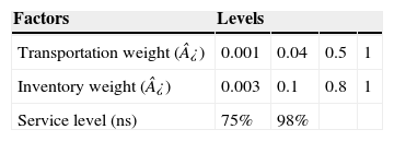
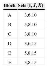
4.2Sensitivity analysisAccording to the characteristics of the supply chain, such as product type, demand, quality, among many others, the decision maker may assign different values to the weights associated to inventory and transportation as well as the service level. So, we changed some parameters in order to know how can this affect. We used the values shown in the Table 4.
The experiment was performed on six different sizes (blocks) with three different cases. Table 5 shows the size of the sets.
To reduce the computation time, we decided to set the preprocessing in C++, which consist of eliminating infeasible subsets of retailers and calculate media and variance of demand as well as the cost of assigning feasible stars. After obtaining the feasible elements, instances were solved using GAMS. Experiment was performedon a PC with 2.49GHz Intel processor and 3.5GB RAM under Windows 2002.
The network configuration, which is our outcome of interest, is defined by the number of open centers and the resulting allocation at both levels of the supply chain. After analyzing the results, we found that the number of distribution centers remains unchanged throughout all runs, so it does not really reflect the influence of the parameters. However, the selected distribution centers and assignments are the decisions affected by the studied parameters.
Since the total cost is weighted, it was necessary to calculate the real cost of the configuration. That is why the three factors were fixed to a unit value, as it was crucial to make the cost comparable regardless of changes in factors. Thus, our response variable is the percentage change in total cost on the best configuration, i.e., the configuration with lower cost.
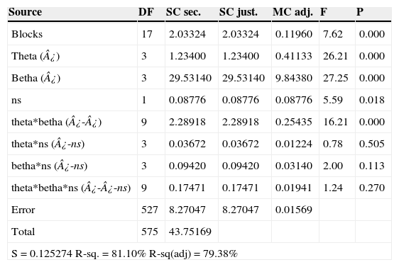
The results were analyzed using Minitab®, special statistical software. Table 6 provides this analysis. The p-value is the probability of being greater than F-stadistic, which is a ratio of the variability between groups compared to the variability within the groups. So, setting a significance level of 0.01, we found that the weighting of transport (¿), the weighting of the inventory (¿) as well as their interaction (¿-¿) are significantly influential in the network configuration. Since the P-value of 0.0 is less than specified significance level of 0.01, the defined values affects the decisions, that is to say, which distribution centers are opened and how to assign retailers, distribution centers and plants.
Analysis of variance.
| Source | DF | SC sec. | SC just. | MC adj. | F | P |
|---|---|---|---|---|---|---|
| Blocks | 17 | 2.03324 | 2.03324 | 0.11960 | 7.62 | 0.000 |
| Theta (¿) | 3 | 1.23400 | 1.23400 | 0.41133 | 26.21 | 0.000 |
| Betha (¿) | 3 | 29.53140 | 29.53140 | 9.84380 | 27.25 | 0.000 |
| ns | 1 | 0.08776 | 0.08776 | 0.08776 | 5.59 | 0.018 |
| theta*betha (¿-¿) | 9 | 2.28918 | 2.28918 | 0.25435 | 16.21 | 0.000 |
| theta*ns (¿-ns) | 3 | 0.03672 | 0.03672 | 0.01224 | 0.78 | 0.505 |
| betha*ns (¿-ns) | 3 | 0.09420 | 0.09420 | 0.03140 | 2.00 | 0.113 |
| theta*betha*ns (¿-¿-ns) | 9 | 0.17471 | 0.17471 | 0.01941 | 1.24 | 0.270 |
| Error | 527 | 8.27047 | 8.27047 | 0.01569 | ||
| Total | 575 | 43.75169 | ||||
| S = 0.125274 R-sq. = 81.10% R-sq(adj) = 79.38% | ||||||
The established service level shows no evidence of impact on the optimal solutions of the model. Regarding cost, service level affects the safety stock, nevertheless it has no influence on the network configuration, not even a large variation as the used here (75–98%). It is due to a satisfactory design is achieved that meet the demand since working inventory and safety stock are large enough.
It is also noted that the blocks (size) have significant influence on the solutions, as expected, since the distribution depends on the number of facilities available in each case (plants, distribution centers, and retailers).
5Conclusion and future workThe importance of the presented work consists on the integration of elements that together have not been addressed in the literature. This integration allows to study more practical situations, but resulted in a much more complex problem, mainly due to the consideration of two levels in the supply chain and the single source constraint involved in thereof. Furthermore, inventory costs involve necessarily nonlinear terms, which make the problem even harder to solve. To avoid the common challenges of nonlinear models we tried a new formulation, however, the resulting model (MILP) has the drawback of an exponentially increase on the number of variables and constraints.
Solving the MINLP model, we could not get optimal solutions and the feasible solutions found were not good. On the other hand, with MILP and BLP models, the solutions found were optimal. Regarding the time required to reach the solutions, the difference between the models is substantial. Preprocessing time is less than optimization time in MINLP model and MILP model, but it is not the case for BLP model, which requires two hours in the largest instance, while its optimization time is the fastest.
Summarizing, thanks to the third model and the preprocessing performed, best results were achieved in reasonable computing time, which shows the appropriateness of devoting efforts to the modeling task.
Although generally linearization is often not obvious and is very time consuming, it may give better results in the long term, especially if you want to achieve optimality and work with cases of large sizes. With these goals, BLP model showed the best results, besides it required less time.
It should be mentioned that the linear models presented are correct only under the assumption of single source suppliers. Considering assumptions like multiple deliveries or multiple suppliers break the structure of the linear models exposed.
In addition we found, from the performed sensitivity analysis, the significant influence of the weights given to transport and inventory in the network configuration, which confirms the importance of considering operational decisions in strategic decision making (opening distribution centers in our case).
It has become clear that solving these models by directly using a commercial optimizer is not viable for large instances. However, the performed experiments allowed us to know the structure of the problem and its behavior, so we intend to apply in the future decomposition techniques, specifically, column generation in order to solve larger cases.
This work was partially supported by the Mexican National Council of Science and Technology (GRANT CB 167019) and Universidad Autonóma de Nuevo León under project IT764-11 PAICYT-UANL. These supports are gratefully acknowledged.