


This paper provides the development of an axial suspended active magnetic bearing (AMB) experimental bench for load and disturbance tests. This test bench must be capable of levitating a 2kg steel disc at a stable working distance of 3mm and a maximum attraction distance of 6mm. The suspension is accomplished by two electromagnets producing upward and downward attraction forces to support the steel disc. An inductive sensor measures the position of the steel disc and relays this to a PC based controller board (dSPACE® controller). The control system uses this information to regulate the electromagnetic force on the steel disc. The intent is to construct this system using relatively low-cost, low-precision components, and still be able to stably levitate the 2kg steel disc with high precision. The dSPACE® software (ControlDesk®) was used for data acquisition. In this paper, an overview of the system design is presented, followed by the axial AMB model design, inductive sensor design, actuating unit design and controller development and implementation. The paper concludes with results obtained from the dSPACE® controller and evaluation of the axial suspended AMB experimental bench with load and disturbance tests.
The project objective is the development of an axial suspended active magnetic bearing (AMB) experimental bench for load and disturbance tests. The system must be constructed by using relatively low-cost, low-precision components and the test bench must provide information on the load and disturbance tests. The development of the experimental bench is the first phase of a larger project on the development of a high performance axial AMB jackhammer for soft use in the residential and industrial sectors. Cases have been reported where cardiac contusion (caused by repeated, less severe blows, over a prolonged period) is caused by the use of jackhammers (Chapman & McEachen, 1957). AMBs in generators, pumps, turbo-machinery, compressors and motors has grown over the last couple of years, because users expect machines to operate at high efficiency and high availability and to be safe and reliable at all times (Gouws, 2012). An AMB provides the advantage of low maintenance cost and high life time, due to the avoidance of lubrication systems and absence of material deterioration and minimal friction losses (Khoo et al., 2010; Ritonja et al., 2006; Schweitzer, Traxler, & Bleuler, 1993). It is therefore important to investigate the use of AMBs in jackhammers, in order to improve safety and increase the life span of jackhammers. An introduction to magnetic bearings and electromagnetic design of a magnetic suspension system is provided by (Allaire & Maslen, 1997; Hurley et al., 1997). It is necessary to perform the following designs to develop the axial suspended AMB experimental bench: (1) axial AMB model design; (2) inductive sensor design; (3) actuating unit design, and (4) controller design. Each of these designs is discussed in detail in this paper.
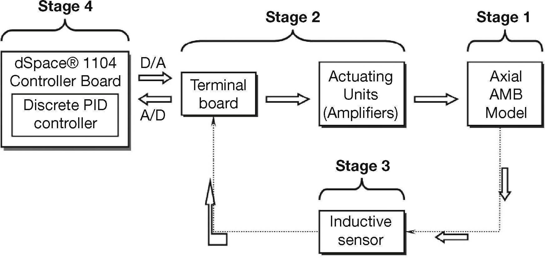
2System DevelopmentThis project can be divided into four stages as shown in Figure 1. Stage 1 focuses on the axial AMB model design. The model consists of a 2kg steel disc and two electromagnets. The one electromagnet will be placed above the steel disc and the other one beneath the steel disc. The steel disc will be connected to a steel rod and will be able to freely move in die axial direction. Stage 2 focuses on the terminal board (which receives signals from the computer and sends them to the actuating units and vice versa) and actuating units (which provides the electromagnets with the correct potential to suspend the disc). The purpose of the terminal board is to isolate the computer from the actuating units and to scale the input and output signals coming from the computer and inductive sensor respectively. Stage 3 focuses on the inductive sensor, which will measure the size of the air gap between the steel disc and the electromagnets. Stage 4 focuses on the design of the discrete PID controller. The dSPACE® 1104 R&D Controller board will be used for this purpose. ControlDesk® (dSPACE® controlling software) is then used to evaluate the system.

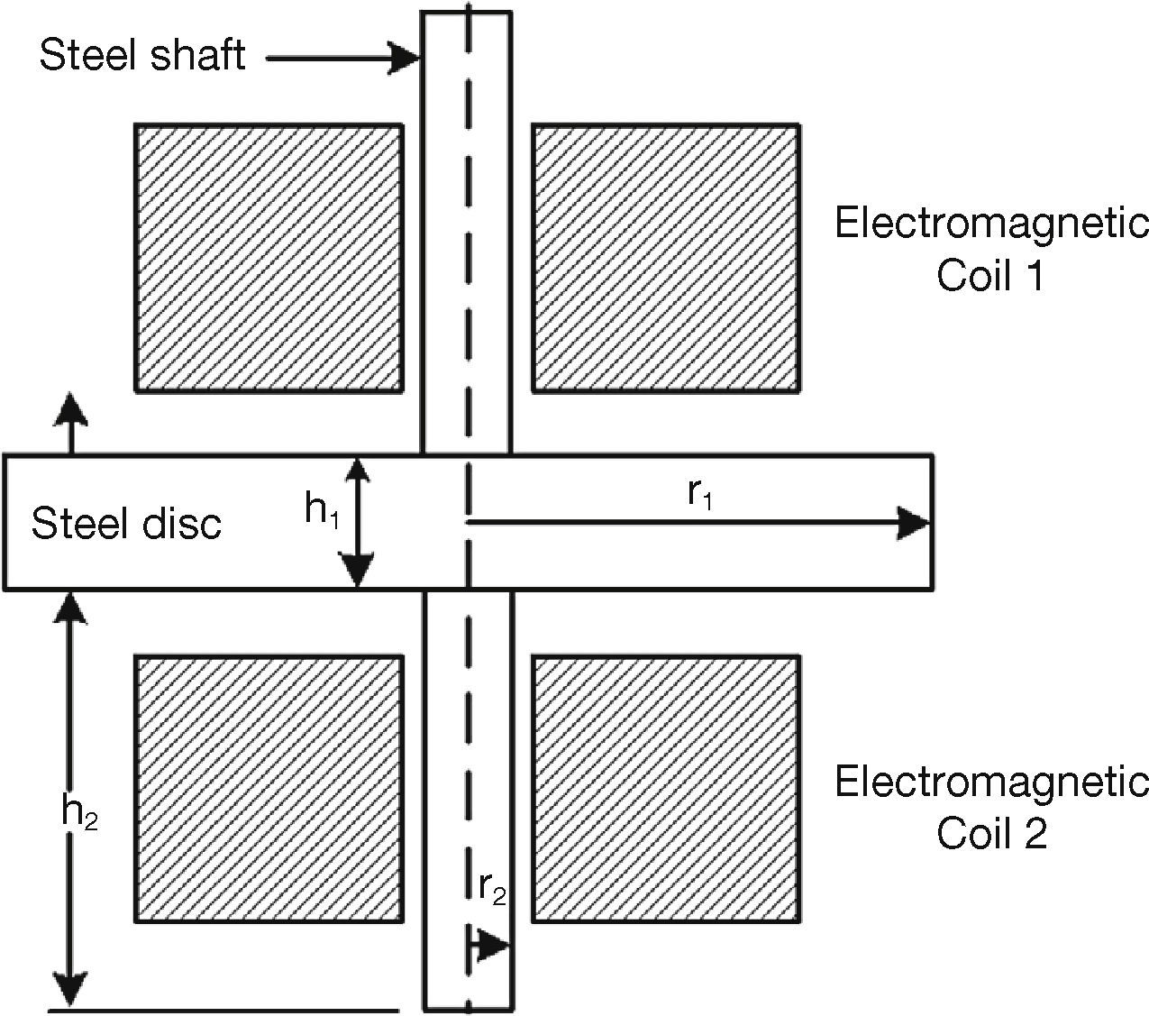
The physical axial AMB model described in this paper constitutes two electromagnets positioned above and beneath a 2kg steel disc with an air gap of 3mm on either side of the disc. The steel disc is not able to move in die radial direction. An inductive sensor is designed to obtain position feedback from the model as can be seen in Figure 2. This sensor measures the size of the air gaps between the suspended steel disc and the electromagnets.

Discrete PID control was used for controlling purposes. The dSPACE® 1104 controller board and software is used for controlling purposes. This paper describes the system development process from the Simulink® model to the real-time model, where the dSPACE® controller board is used to control the physical hardware.
The dSPACE® controller sends out control signals via D/A ports to the actuating units. The actuating units then provide controlling currents to the electromagnets. The steel disc is attracted or released according to the signals provided. The design of a state observer (using the Luenburger observer technique) for position control of a DC servo motor is presented by Sawant and Ginoya (2010). The implementation is done on the dSPACE® DSP DS-1104 controller board and the control scheme is designed using the pole placement technique (Sawant & Ginoya, 2010).
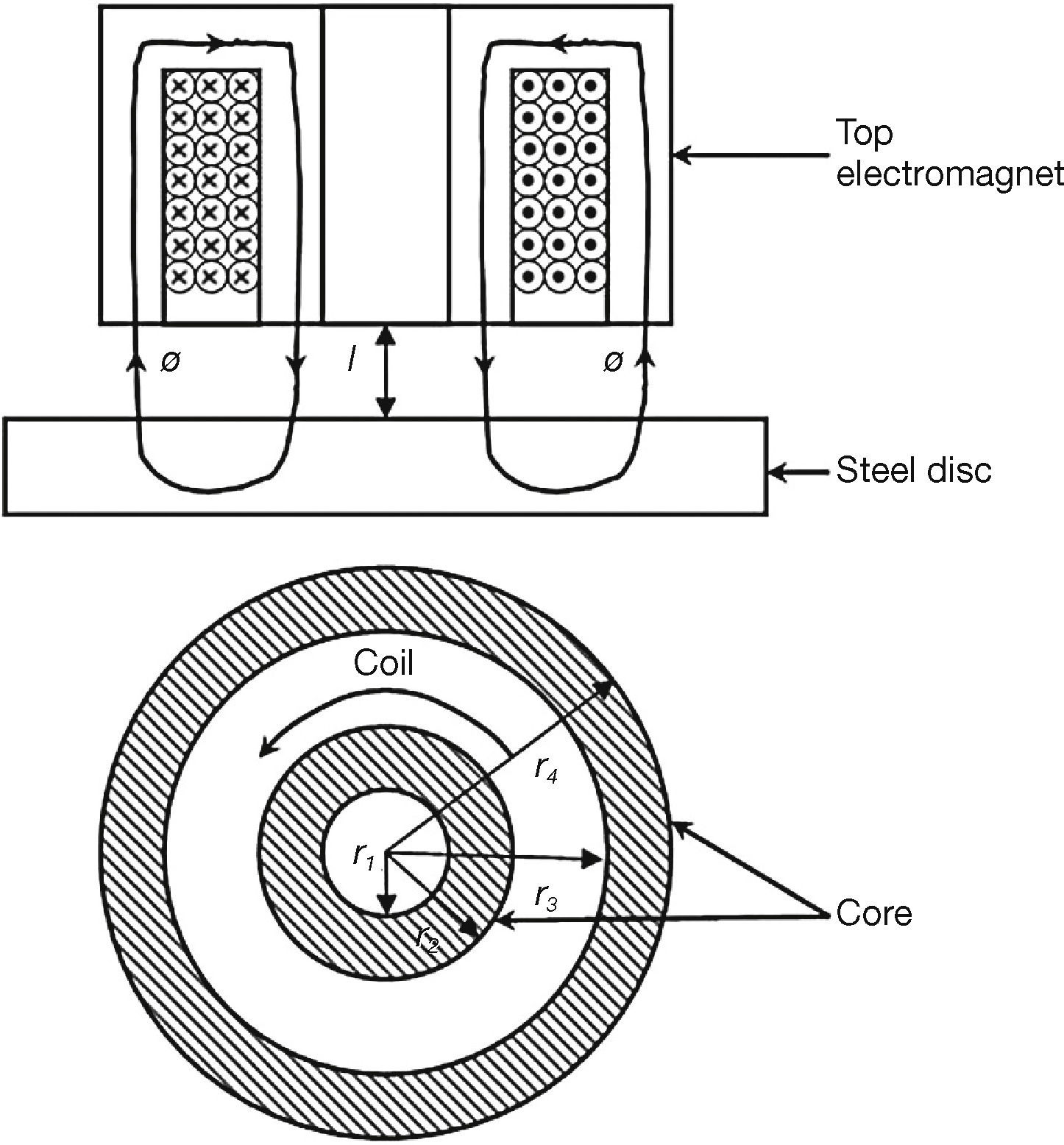
3Axial AMB Model DesignWhen starting an axial AMB model design, it is important to know the specifications of the model. The model must be designed to suspend a 2kg steel disc at a working distance of 3mm with a maximum attraction distance of 6mm. Next, it is important to obtain the core dimensions, since the model specifications together with the core dimensions will be used to obtain the theoretical design parameters of the model. A layout of the core can be seen in Figure 3.

The gravitational force (F) required to lift the rotor is provided by:

The purpose of the electromagnet is to apply a force on the rotor to maintain a constant air gap between the rotor and the stator (Kasarda, 2000; Gouws, 2013a). The air gap flux (ø) required to lift the rotor is determined by using Eq. (2):

where μ0 is the permeability of free space; Ai is the inner core area given by Ai = π(r22–r21), and Ao is the outer core area given by Ai = π(r24–r23).
The total magneto-motive force (F) required to set up the desired flux in the air gap is given by Eq. (3):
where øt is the total flux, and Rt is the total reluctance.
A current of 1 A was chosen since it can be easily supplied.
The current density (J) in the wire was safely chosen at 3 A/mm2. The diameter of the wire dw can thus be calculated by using Eq. (4):

To determine the steady state voltage needed for the electromagnet to operate, the resistance of the copper in the coil has to be determined. The current at which the magnet will operate have already been specified thus the required voltage can be determined using Ohm's law. The number (N) of turns in the coil can be determined by using Eq. (5):
The resistance of the wire is determined by using Eq. (9), therefore the length of the wire (lw), cross sectional area (Aw) and the electrical resistivity of copper (ρc) has to be calculated before the resistance of the wire can be calculated. The length of the wire (lw) required is calculated by using Eq. (6):
where Cave is the average circumference of the coil given by Cave = 2πrave.
The cross sectional area (Aw) of the wire is calculated by using Eq. (7):
where rw is the radius of the wire given by rw = 1/2 dw.
The resistivity of copper can be calculated by using Eq. (8):
where ρ0 is the resistivity at temperature T; T is the assumed temperature of 50°C, and αc is copper temperature coefficient of resistivity.The resistance of the coil is then given by Eq. (9):
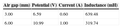
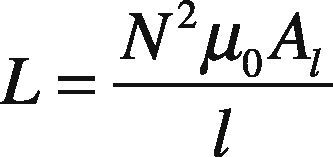
The inductance (L) of the electromagnet is determined by using Eq. (10):
The potential, current and inductance at different air gaps can then be determined. Table 1 provides a summary on the steady state values.
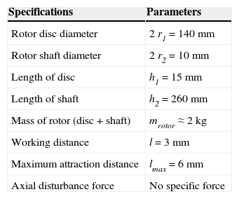
The design process is done iteratively until the desired value for the force, number of turns in the coil and dimensions of the electromagnet have been reached. Table 2 provides a summary of the model specifications showing the length (h1 and h2) and diameter (r1 and r2) of the disc and shaft.
Summary of the model specifications.
| Specifications | Parameters |
|---|---|
| Rotor disc diameter | 2 r1 = 140 mm |
| Rotor shaft diameter | 2 r2 = 10 mm |
| Length of disc | h1 = 15 mm |
| Length of shaft | h2 = 260 mm |
| Mass of rotor (disc + shaft) | mrotor ≈ 2 kg |
| Working distance | l = 3 mm |
| Maximum attraction distance | lmax = 6 mm |
| Axial disturbance force | No specific force |
More information on electromagnetic model design and magnetically suspended flywheel energy storage devices are provided (Ahrens, Kucera, & Larsonneur, 1996).
4Inductive Sensor DesignThe inductive sensor measures the size of the air gap and provides position feedback. The sensor must be designed to show a linear response between the position and the output voltage at the operating point of the AMB. Furthermore, it must have low noise susceptibility and low temperature dependence.
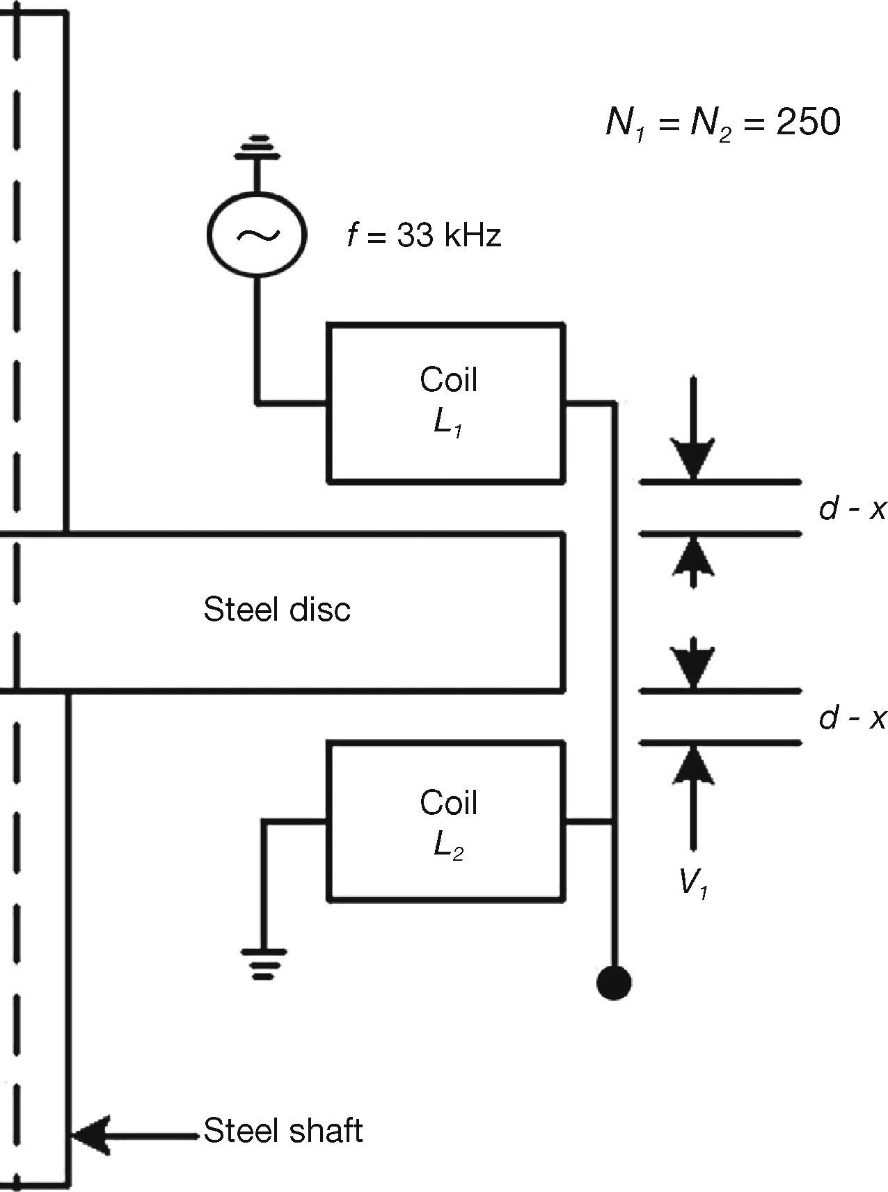
The inductive sensor configuration used to measure the position of the steel base is shown in Figure 4. The inductances L1 and L2 are functions of the air gap size, where (Pretorius, 1982):


and
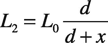
This change in inductance will be used to obtain a change in the position sensor output voltage.
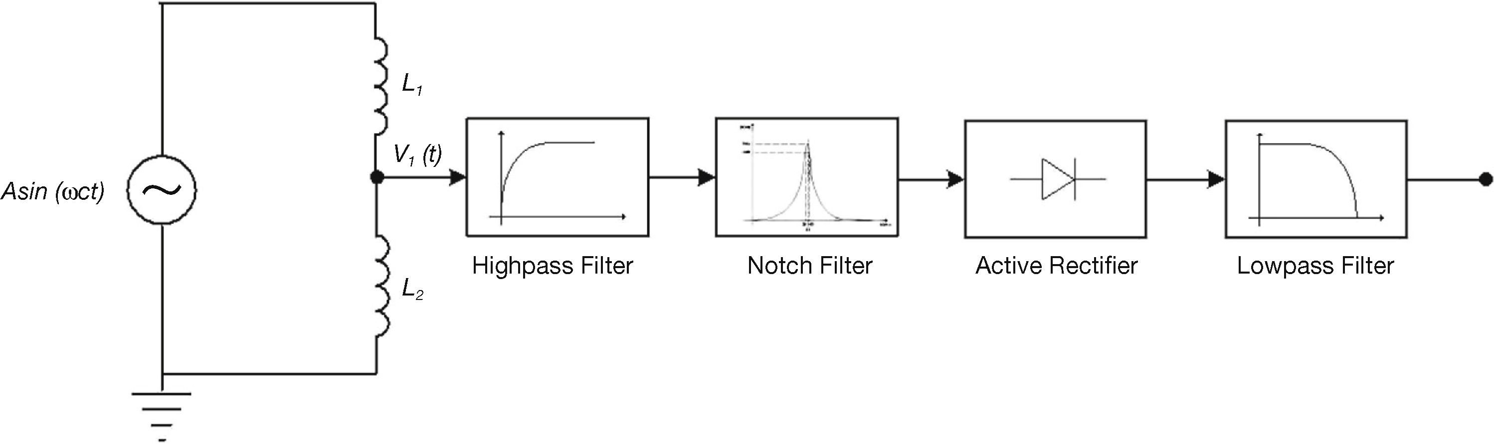
The sensor functional block diagram is shown in Figure 5. A sinusoidal signal generated by an oscillator is applied across the two sensor inductors connected as a voltage divider. A difference in the inductance of L1 and L2 provides a difference in the amplitude of the output signal v1(t). The amplitude of v1(t) increases when L2 > L1 and decreases when L1 > L2.

The signal v1(t) is fed through a second order Butterworth high pass filter, filtering all the low frequency noise induced by the coils and power supplies. Since the position sensor coils and the electromagnets are located in close proximity, electromagnetic interference can occur. This problem is solved by using a Butterworth band pass filter (notch filter).
The position signal is passed through the notch filter, while any noise from the electromagnetic coil is filtered. A Butterworth filter is used, because it has a flat amplitude response in the pass-band and a steep cut-off response in the stop band (Pretorius, 1982). The Butterworth band pass filter is designed to have as flat as possible frequency response in the pass-band. A Butterworth band-pass filter is obtained by inserting an inductor in parallel with each capacitor and a capacitor in series with each inductor to form a resonant circuit. Each new component resonates with the old component at the selected frequency (Bianchi & Sorrentino, 2007).
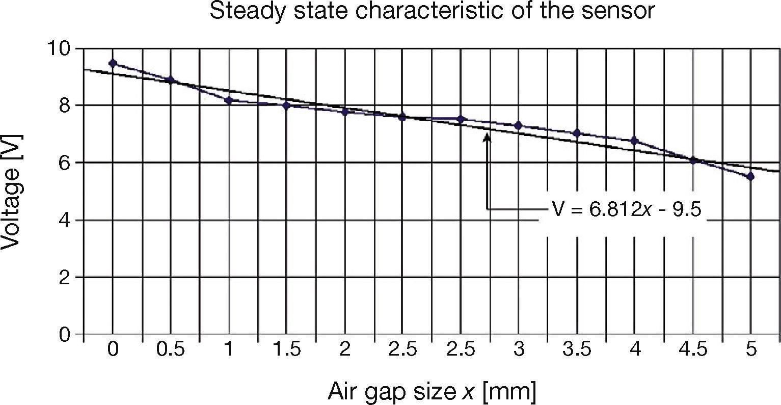
The active rectifier functions as an ideal peak detector and provides a DC output. A low pass filter (fa ≈ 1kHz) and difference amplifier can be used to filter out any high frequencies and to centre the output on zero. The typical transfer characteristic of the inductive sensor is shown in Figure 6. The linear area can be improved by using a full-wave active rectifier instead of a half-wave active rectifier and obtaining the optimum inductance for the desired air gap. This optimum inductance can be obtained from Eq. (11-12).
5Actuating Unit Design
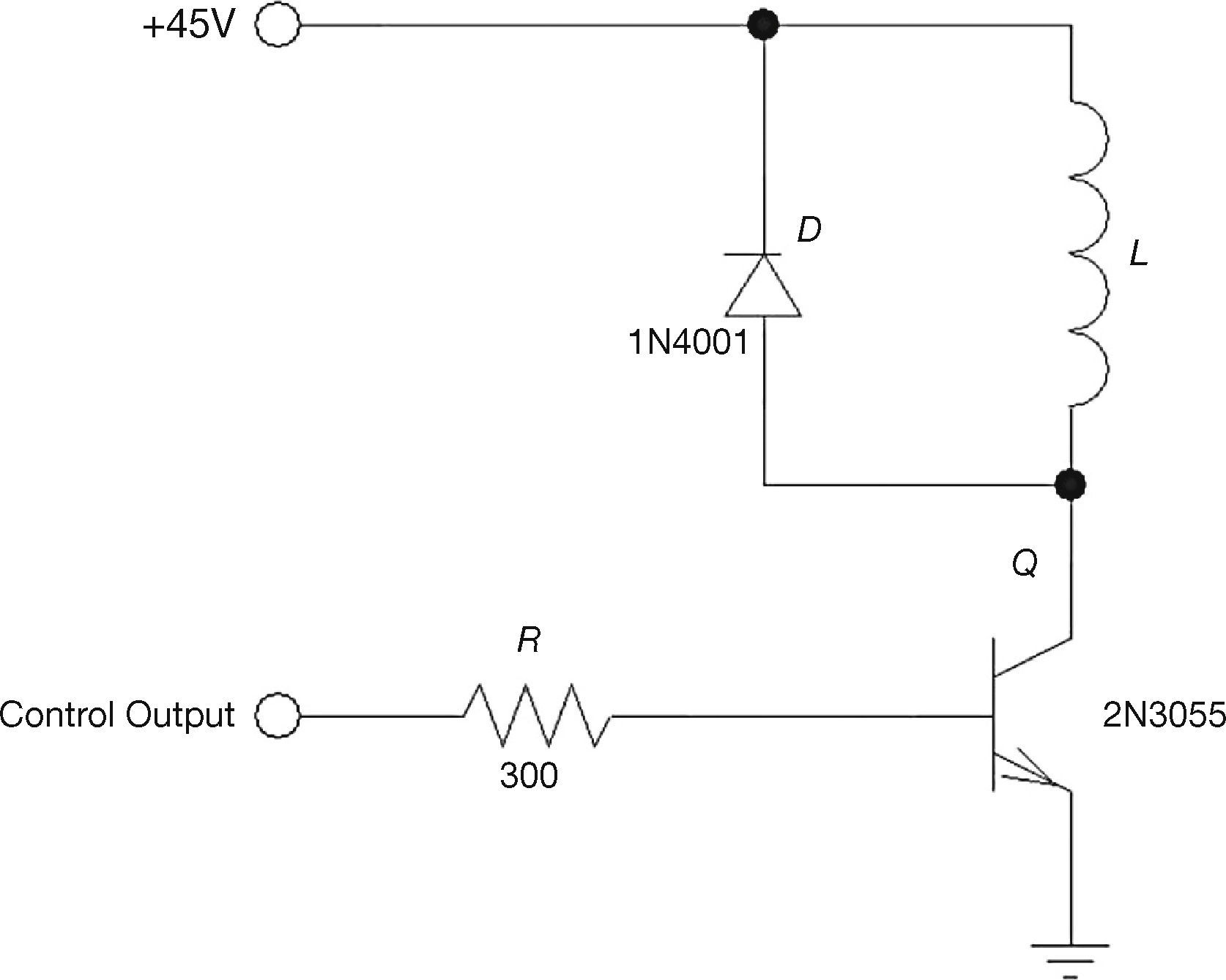
A linear voltage amplifier is used as an actuating unit. The circuit in Figure 7 controls the current in the electromagnetic levitation coil L. It is driven by an op-amp, which is specified to source up to 40mA of current. The 2N3055 transistor has a beta of more than 50, which is sufficient to drive loads of up to 2 A without any additional circuitry.

The base resistor (R) provides current protection and limits the output current demand on the op-amp. The supply voltage of the op-amp is 12V and the base terminal voltage is 0.7V. Therefore the maximum base current (Ib) is 37.67mA. The actual maximum value of the base resistor that can be used depends on the maximum collector current required and the gain (beta) of the transistor.
The diode (D) is connected in parallel with the coil and provides a freewheeling path for the inductor current when the transistor turns off.
6Controller Development and ImplementationThis system is highly nonlinear and is normally linearized at an operation point for control analysis. The force can be determined by using Eq. (13) (Antsaklis & Gao, 2005):

where Fe is the external disturbance force; ki is the current gain; ks is the position stiffness, and x is the air gap.
This system has only one PD controller and can be represented as an equivalent spring-mass-damper system as follows (Gouws, 2013b):
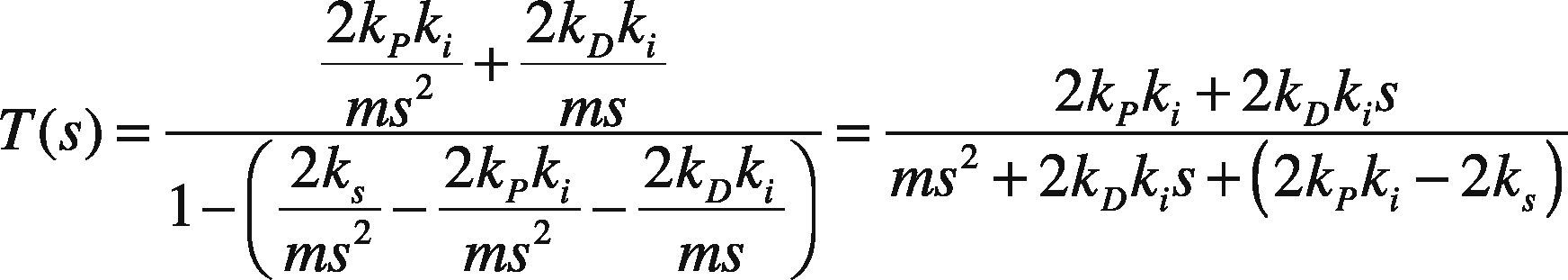
where kD is the derivative gain, and kP is the proportional gain.
From Eq. (14), the equivalent spring-mass-damper characteristic equation is provided by (Alaire et al., 1997):
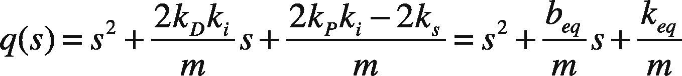
where s2+beqms+keqm is the standard form of the spring-mass-damper equation.
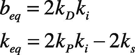
The equivalent damping constant (beq) and stiffness (keq) is thus (Scherpen, 1998):
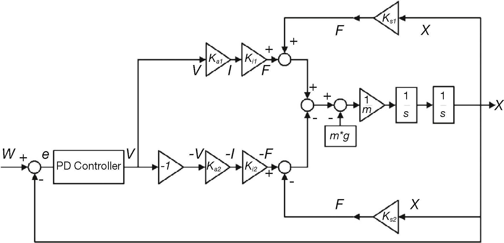
The linearized AMB system with a PD controller can be represented by the block diagram in Figure 8. The parameters ka1 and ka2 are current to voltage gains, while the parameters ki1 and ki2 are the attraction force to current gains. The parameters ks1 and ks2 are the attraction force to air gap gains. The constants of the PD controller can be calculated by using Eq. (16). The parameter for the open loop stiffness (ks) of the model can be determined by using Eq. (17) (Sinha, 1987; Gouws, 2013c):
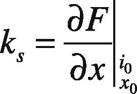

where F is the attraction force of the electromagnet and x is the air gap size.
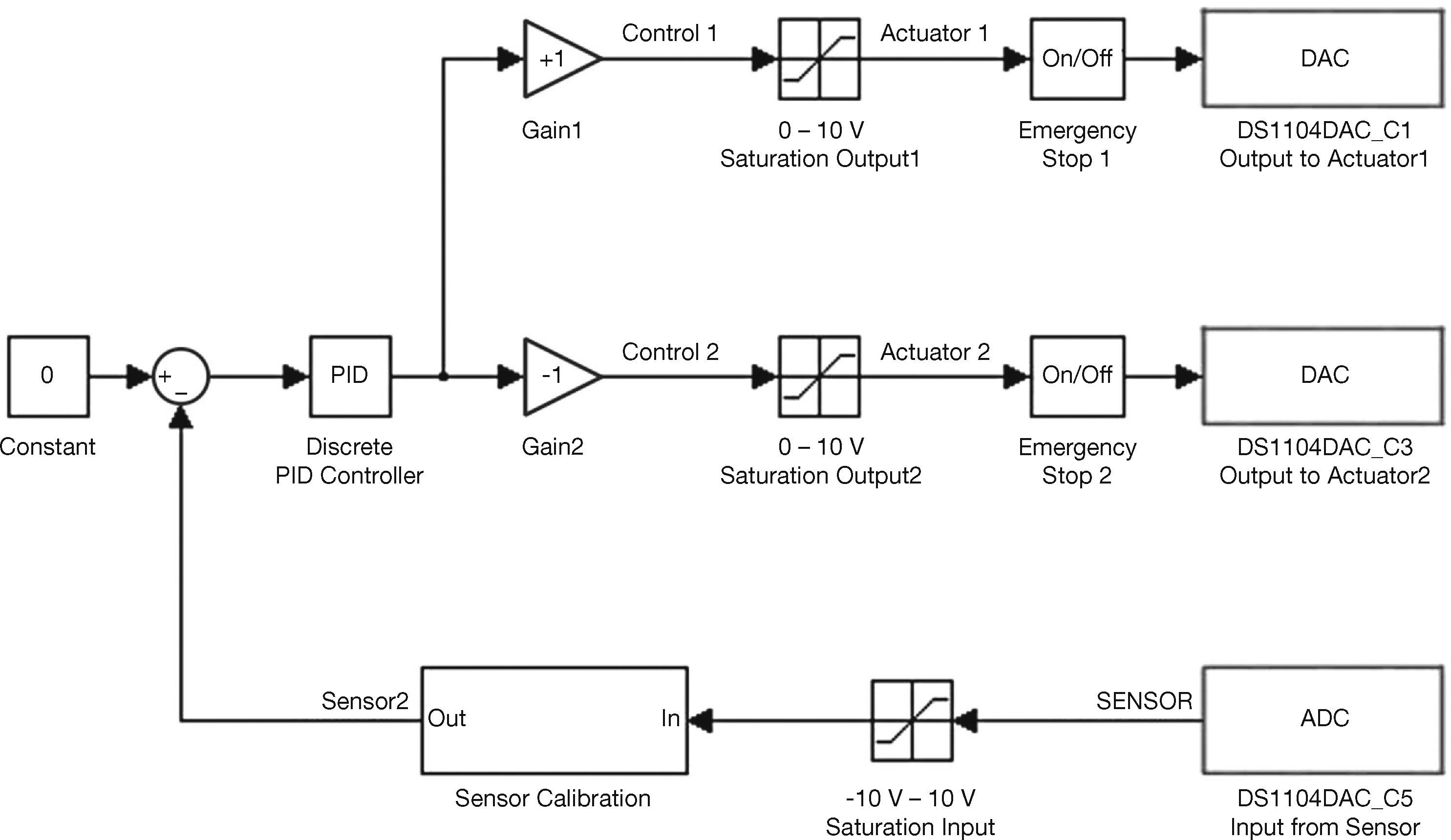
The value of the proportional gain (kP) is adjusted to realize the required stiffness, then the value of derivative gain (kD) is adjusted to realize the required damping. Finally the integrator is implemented such that τD < τi/10. An integrator is implemented in the experimental system to obtain a smaller steady state error. A real time model can be created after the constants of the controller have been determined. Figure 9 shows the real time Simulink® model.

It was decided to choose the sample time (Ts) of the real time interface (RTI) at least 7 times the bandwidth of the sensor. The bandwidth of the sensor is ≈ 1kHz, therefore fsreal_time > 7kHz. The sample time was chosen at Tsreal_ time = 0.0001 s (fsreal_ time = 10 kHz).
The sensor signal enters the dSPACE® controller at ADC port 5 as can be seen in Figure 9. Upper and lower limits of –10V and +10V are placed on the signal and the signal is then passed onto the sensor calibration block, where the gain and level of the sensor signal is adjusted.
The signal “sensor2” is subtracted from the position reference of the model. The steel disc can be moved up and down by changing the value of the position reference. This signal is then passed onto a discrete PID controller, from where it is sent to the different actuator stages.
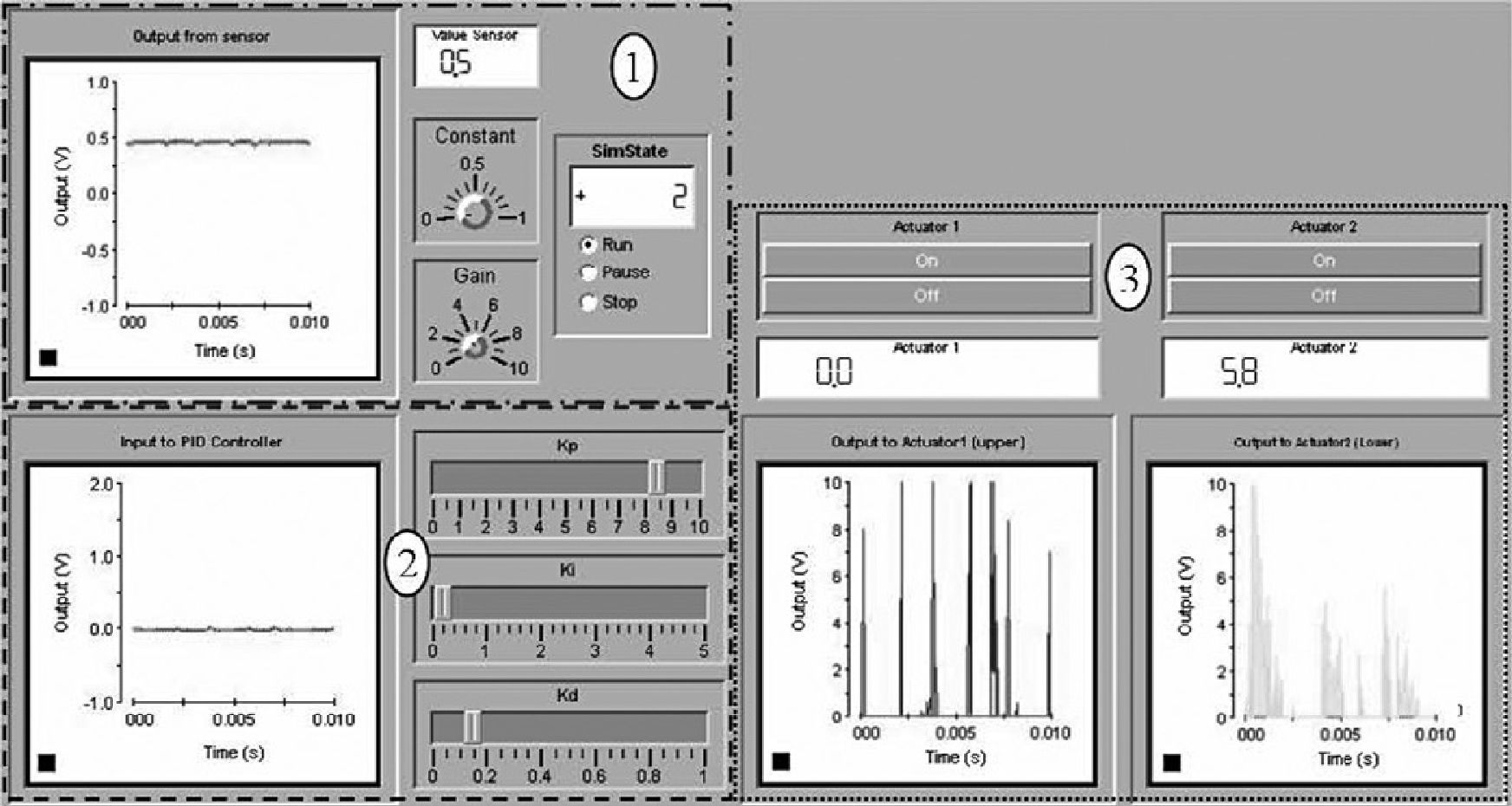
A lower limit of zero has been placed on “Control1” and “Control2” to prevent negative output values. Emergency stop blocks have been inserted on the different actuator stages. Actuator 1 and 2 receives signals from DAC ports 1 and 3 respectively. After the real time model, as shown in Figure 9, has been created, the ControlDesk® interface must be created. This interface will be used for real time data acquisition. A preview of a ControlDesk® interface can be seen in Figure 10.

Section 1 in Figure 10 shows all the real time information regarding the sensor. A graph of the output of the sensor can be seen in the upper left corner. Sensor calibration is done by adjusting the constant and gain knobs. A digital output of the sensor voltage can also be seen in this section. The real time simulation can be stopped or paused at any time by means of the SimState block.
Section 2 shows all the real time information regarding the PID controller. This section shows a graph of the input signal to the controller and the scroll bars for the parameters kP, ki and kD of the PID controller.
Section 3 shows all the real time information regarding actuator 1 and actuator 2. Graphs of the output to actuator 1 and 2 can be seen in the lower left corner. Displays showing the voltage output of actuator 1 and 2 and on and off pushbuttons for the different actuators can also be seen in this section.
After the ControlDesk® interface has been created, the real time Simulink® model of Figure 9 is downloaded onto the dSPACE® controller board. The ControlDesk® interface can then be used to capture information, change the PID constants in real time and calibrate the sensor in real time.
The development of HIL setup for collision avoidance of an under-actuated flat-fish type AUV using ControlDesk® experiment software and the dSPACE® DS1104 R&D controller is presented by Subramanian et al. (2012). The results show that the developed collision avoidance algorithm can be used in real-time for the flat-fish type AUV and dSPACE® HIL setup is an effective tool for the verification of control algorithms (Subramanian et al., 2012).
7Evaluation of the SystemThe following three tests were performed on the experimental AMB system: (1) load test; (2) disturbance test, and (3) system output with variation in input step response.
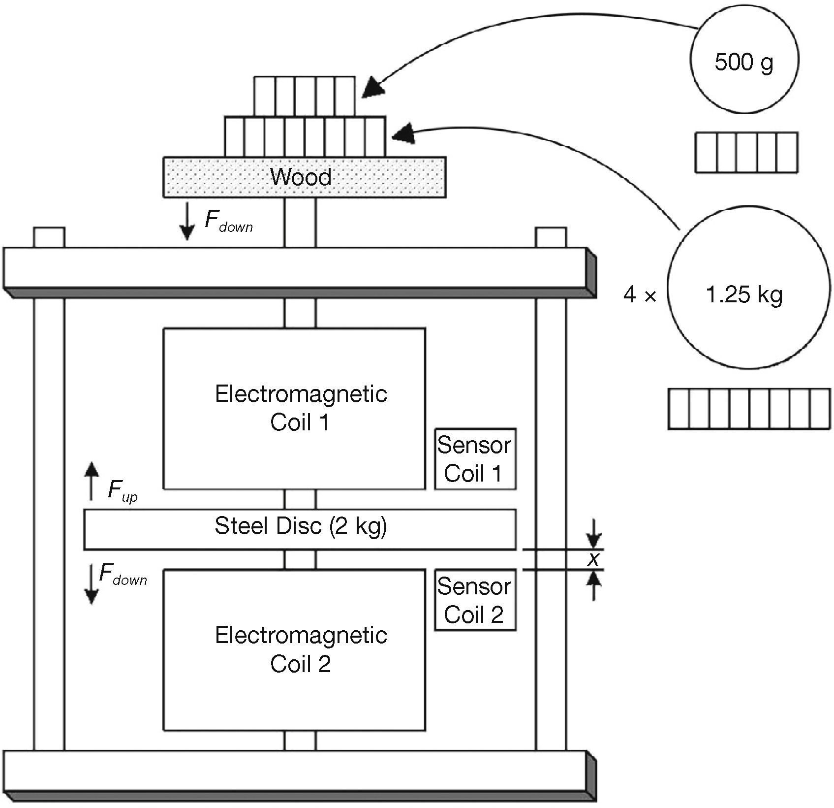
7.1Load Test Performed on the ModelThe load test was conducted by placing different size weights on top of the steel rod of the model and to observe what impact the downward force (Fdown) of the weights has on the amount of current necessary to keep the steel disc in suspension.
For this test, the reference air gap (x) is chosen between the steel disc and the bottom electromagnet (as seen in Fig. 11). Four 1.25kg weights and one 500g weight were placed on the model. Table 3 provides the data obtained with the load test.

Data obtained with the load test.
| Mass (kg) | Top electromagnet current (A) | Air gap x (mm) | Steady state error ess (mm) | |||||||||
|---|---|---|---|---|---|---|---|---|---|---|---|---|
| Analog Lead | Discrete Lead | Analog PID | Discrete PID | Analog Lead | Discrete Lead | Analog PID | Discrete PID | Analog Lead | Discrete Lead | Analog PID | Discrete PID | |
| {2 kg steel disc} | 0.31 | 0.50 | 0.65 | 0.80 | 3.00 | 3.00 | 3.00 | 3.00 | 0.00 | 0.00 | 0.00 | 0.00 |
| 0.50 | 0.35 | 0.70 | 0.80 | 1.00 | 3.00 | 3.00 | 3.00 | 3.00 | 0.00 | 0.00 | 0.00 | 0.00 |
| 1.25 | 0.42 | 0.90 | 0.97 | 1.40 | 2.90 | 2.90 | 3.00 | 3.00 | 0.10 | 0.10 | 0.00 | 0.00 |
| 2.50 | 0.55 | 1.20 | 1.15 | 1.70 | 2.40 | 2.50 | 3.00 | 3.00 | 0.60 | 0.50 | 0.00 | 0.00 |
| 3.75 | 0.73 | 1.50 | 1.55 | 2.10 | 1.50 | 1.60 | 2.90 | 2.90 | 1.50 | 1.40 | 0.10 | 0.10 |
| 5.00 | 0.98 | 1.70 | 1.79 | 2.50 | 0.00 | 0.00 | 0.00 | 0.00 | 3 (∞) | 3 (∞) | 3 (∞) | 3 (∞) |
From this table, it can be seen that the steady state error stays zero for all the controllers up to an added mass of 0.5kg. The steady state error for the PID controllers stays zero up to an added mass of 2.5kg. When the weight increases to 5kg, the steady state error increases to 3mm. The steel disc at this stage lies on top of the bottom electromagnet.
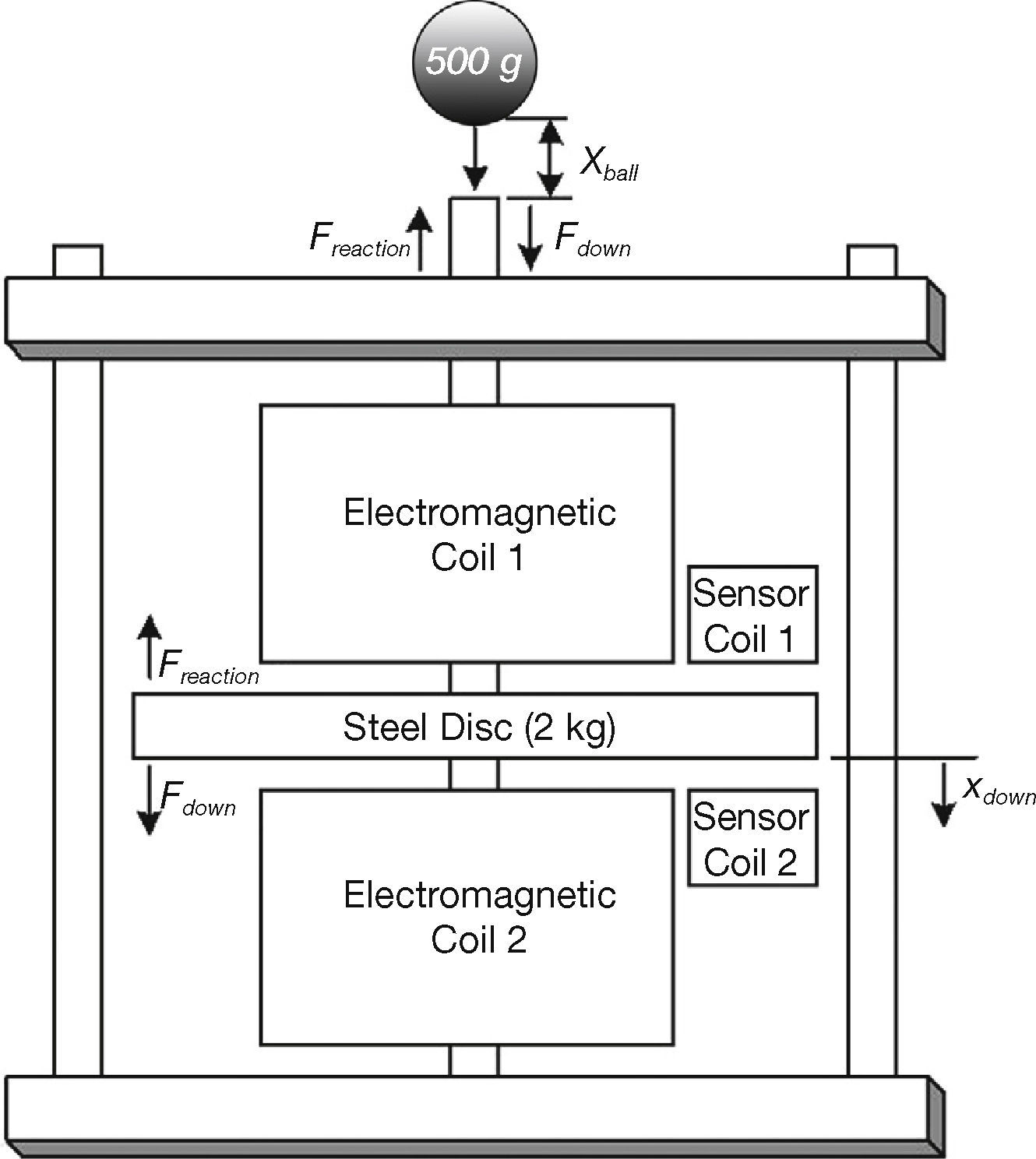
7.2Disturbance Test Performed on the ModelIn Figure 12, the system is evaluated by applying disturbance forces on it. A 500g ball falling from different heights is used as disturbance on the system to see if the system can recover from the disturbance force and stably suspend the disc again.

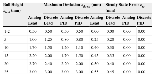
The ball falls from a distance defined as xball, which provides a downward disturbance force of Fdown and a reaction force of Freaction. The downward deviation of the steel disc is defined by xdown. Figure 12 illustrates the disturbance test setup. Table 4 provides the disturbance output of the system with a ball falling from different heights. The maximum deviation and steady state error stays the same for all the controllers when the height of the ball is between 1 and 2mm.
Data obtained with the disturbance test.
| Ball Height xball (mm) | Maximum Deviation xdown (mm) | Steady State Error ess (mm) | ||||||
|---|---|---|---|---|---|---|---|---|
| Analog Lead | Discrete Lead | Analog PID | Discrete PID | Analog Lead | Discrete Lead | Analog PID | Discrete PID | |
| 1-2 | 0.50 | 0.50 | 0.50 | 0.50 | 0.00 | 0.00 | 0.00 | 0.00 |
| 5 | 1.00 | 1.25 | 0.80 | 0.80 | 0.25 | 0.20 | 0.00 | 0.00 |
| 10 | 1.70 | 1.50 | 1.20 | 1.10 | 0.40 | 0.30 | 0.00 | 0.00 |
| 15 | 2.20 | 2.00 | 1.70 | 1.50 | 0.45 | 0.35 | 0.00 | 0.00 |
| 20 | 2.70 | 2.40 | 2.20 | 2.00 | 0.50 | 0.40 | 0.00 | 0.00 |
| 25 | 3.00 | 3.00 | 3.00 | 3.00 | 0.55 | 0.45 | 0.00 | 0.00 |
When the ball falls from a height of 25mm, the steady state errors for the PID controllers are zero. The steel disc at this stage is hammered down onto the bottom electromagnet.
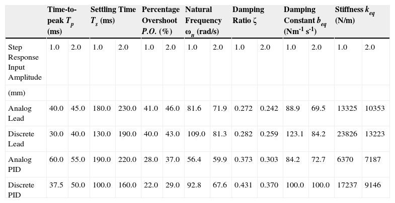
7.3System Output With Variation in Input Step ResponseIn this section, the AMB system will be evaluated as a spring-mass-damper system. The following equations were used to determine the natural frequency (ωn), settling time (Ts) and time-to-peak (Tp):
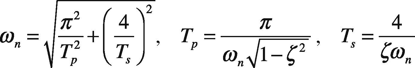
where ζ is the damping ratio.
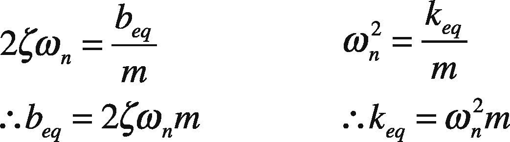
The damping constant (beq) and stiffness (keq) of the model can be determined by using Eq. (19):
The results of the system output with variation in input step response amplitude can be seen in Table 5. This table provides information about the system output for the different controllers.
System output with variation in input step response amplitude.
| Time-to-peak Tp (ms) | Settling Time Ts (ms) | Percentage Overshoot P.O. (%) | Natural Frequency ωn (rad/s) | Damping Ratio ζ | Damping Constant beq (Nm-1 s-1) | Stiffness keq (N/m) | ||||||||
|---|---|---|---|---|---|---|---|---|---|---|---|---|---|---|
| Step Response Input Amplitude | 1.0 | 2.0 | 1.0 | 2.0 | 1.0 | 2.0 | 1.0 | 2.0 | 1.0 | 2.0 | 1.0 | 2.0 | 1.0 | 2.0 |
| (mm) | ||||||||||||||
| Analog Lead | 40.0 | 45.0 | 180.0 | 230.0 | 41.0 | 46.0 | 81.6 | 71.9 | 0.272 | 0.242 | 88.9 | 69.5 | 13325 | 10353 |
| Discrete Lead | 30.0 | 40.0 | 130.0 | 190.0 | 40.0 | 43.0 | 109.0 | 81.3 | 0.282 | 0.259 | 123.1 | 84.2 | 23826 | 13223 |
| Analog PID | 60.0 | 55.0 | 190.0 | 220.0 | 28.0 | 37.0 | 56.4 | 59.9 | 0.373 | 0.303 | 84.2 | 72.7 | 6370 | 7187 |
| Discrete PID | 37.5 | 50.0 | 100.0 | 160.0 | 22.0 | 29.0 | 92.8 | 67.6 | 0.431 | 0.370 | 100.0 | 100.0 | 17237 | 9146 |
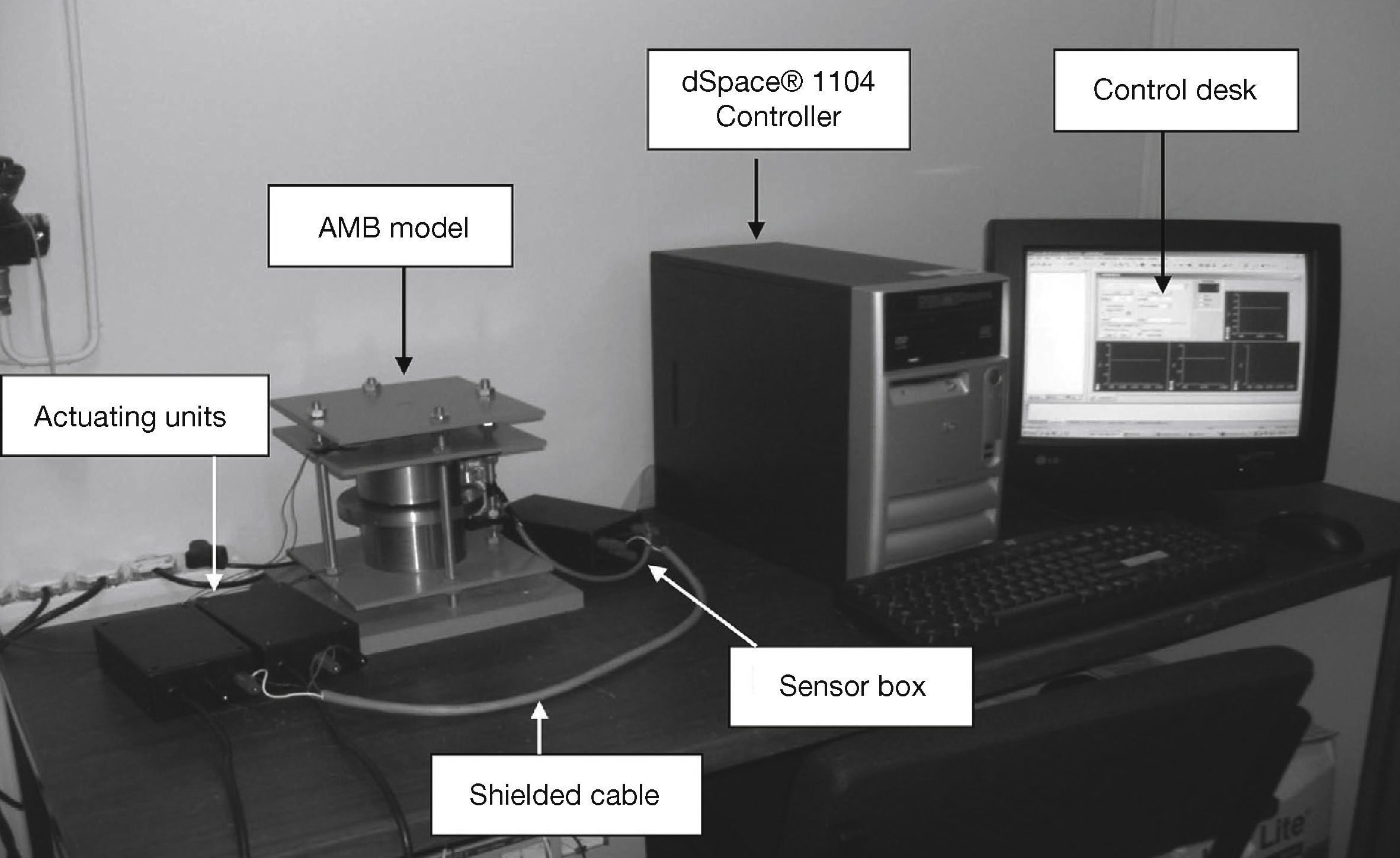
A photo of the complete AMB system showing the actuating units, AMB model, inductive sensor box, dSPACE® 1104 controller and ControlDesk® software interface can be seen in Figure 13.

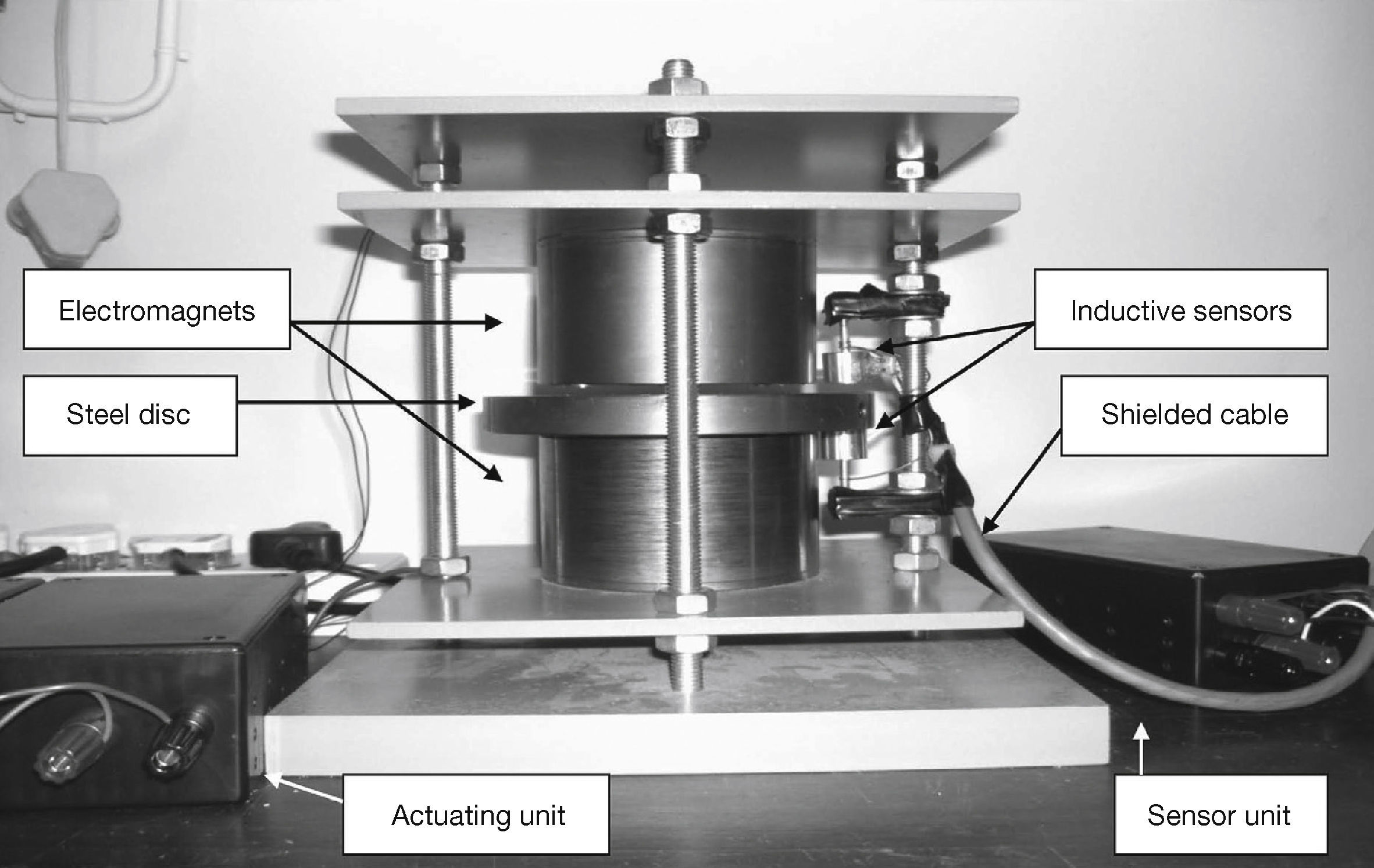
A photo of the complete axial AMB model showing the steel disc, electromagnets, inductive sensors, sensor unit and actuating unit can be seen in Figure 14.

Various other papers on active vibration control in a rotor system, vibration analysis of rolling element bearings defects and mechatronic design and dynamic modeling provides interesting further reading (Arias-Montiel, Silva-Navarro, & Antonio-García, 2014; Saruhan, Sarıdemir, Çiçek, & Uygur, 2014; Mendoza-Bárcenas, Vicente-Vivas, & Rodríguez-Cortés, 2014).
9ConclusionsFor this project, an axial suspended AMB experimental bench for load and disturbance tests was developed. This project is the first phase of a larger project on the development of a high performance axial AMB jackhammer for soft use in the residential and industrial sectors. The advantage of this project lays in the results obtained from the experimental developed system which was constructed by using relatively low-cost, low-precision components. The developed system provides results on different load conditions, different disturbance conditions and variation in input step response conditions.
From the load test with the PID controllers, it can be seen that the steady-state error (ess) remains zero up to an added mass of 2.5kg. From the steady state error obtained during the load test, the conclusion can be made that the PID controller is the better controller, since it has a smaller steady state error. The lead controller also suspends the disc, but has a larger steady state error.
From the disturbance test with the PID controllers it can be seen that the steady-state error remains zero when a ball causing a disturbance at a height of 25mm. From the data obtained for the disturbance test, the conclusion can be made that the PID controller is also the better controller (in terms of the ess). The lead controller recovers from the disturbance, but has a larger steady state error.
From the input step response test, the analog lead controller provides the advantage of the lowest damping ratio (ζ) and the lowest damping constant (beq) for a 2mm input step response. The discrete lead controller provides the advantage of the fastest time-to-peak (Tp) for a 2mm input step response. The analog PID controller provides the advantage of the lowest natural frequency (ωn) and lowest stiffness (keq) for a 2mm input step response. The discrete PID controller provides the advantage of the fastest settling time (Ts) and lowest percentage overshoot (P.O.) for a 2mm input step response.
Higher values of the damping ratio and natural frequency results in higher damping constant values for that specific controller. This can be seen from the values of the discrete PID controller, which has the highest damping constant value for a 2mm input step response. Higher natural frequency values result in higher stiffness values for that specific controller. This can be seen from the discrete lead controller, which has the highest stiffness value for a 2mm input step response.
It was necessary to perform the following designs to develop the axial suspended experimental bench: (1) axial AMB model design; (2) inductive sensor design; (3) actuating unit design, and (4) controller design. The dSPACE® controller and software makes it easier to establish a real time link between the physical AMB model and the discrete controllers, with the advantage of data acquisition and parameter changing in real time. The performance of the AMB system can further be improved by means of advanced control techniques like fuzzy logic control (Ciocirlan, Marghitu, Beale, & Overfelt, 1998), sliding mode control (Allaire & Sinha, 1998) and H∞ control (Djouadi & Tsiotras, 1999).
One of the most effective and efficient modern custom power devices used in power distribution networks to mitigate power quality problems, such as voltage swell and voltage sag, is dynamic voltage restorer (DVR) (Shitole & Gopalakrishnan, 2012). The implementation of the control and detection algorithm of DVR in the dSPACE® (DS1104) real time simulator is presented by Shitole and Gopalakrishnan (2012).