Distributed PSO Algorithm for Data Model Partitioning in Power Distribution Systems

Abstract

This paper presents a method for data model partitioning of power distribution network. Modern Distribution Management Systems which utilize multiprocessor systems for efficient processing of large data model are considered. The data model partitioning is carried out for parallelization of analytical power calculations. The proposed algorithms (Particle Swarm Optimization (PSO) and distributed PSO algorithms) are applied on data model describing large power distribution network. The experimental results of PSO and distributed PSO algorithms are presented. Distributed PSO algorithm achieves significantly better results than the basic PSO algorithm.

1

Introduction

The trend to integrate a power distribution system with other systems within the Smart Grid (SG), effects on expanding the functionality of the Distribution Management System (DMS) [1, 2]. It also expands the data model of the distribution network. This extension applies not only to increase the amount of data (which types are already present in the model), but also to increase the granularity (the introduction of new types of data) [3, 4] - eg. the introduction of “smart” meters in the AMI subsystems, management of energy use in the home systems (HAN subsystem), and others. In this way a large amount of data from the field are presented. It increases the operational efficiency of DMS systems and provides more data to other subsystems within the SG system. Integration with GIS systems expands the data model with geographic data, and the introduction of new (renewable) energy sources in distribution networks [1] can greatly change the topological structure of the network and increase the complexity of most analytical power calculations [5]. In addition, specified analytic functions (eg Topology Analyser (TA), Load Flow (LF), State Estimation (SE), Fault Calculation (FC), Performance Indices (PI), Volt/Var Control (VVC), etc.) will be used more frequent within the SG system and should be extended to the low-voltage part of the network to the individual consumer.

Based on the above, it can be concluded that in the modern SG system of amounts of data, which are under the jurisdiction of the DMS system, increase significantly. Furthermore, the analytical power functions are performed more complexly and more frequently. Integration and communication with other subsystems within the SG system additionally affects the DMS system, so it is necessary to find a solution to decrease the pressure on the system in conditions of frequent execution of analytical functions. The most acceptable solution is to divide the data model into parts, over which the calculations are carried out independently and to perform calculations in parallel.

The problem of data model partitioning can be reduced to the problem of weighted graph partitioning. In addition, graph vertices are subsets of data corresponding to the maximum independent calculation regions. For most analytical power functions (e.g., LF, SE, VVC, et al.) calculation regions are roots (groups of electrical elements powered from the same source). The quantitative measures of the connection between the roots can be the number of the open switch equipment between the roots (tie switches). Therefore, graph edges represent open switches between elements from different roots. The weight of the vertex is determined by the calculation complexity of the corresponding root and the weight of edge are defined as the number of open switches between the corresponding roots [6].

The problem of graph partitioning is NP complete problem [7]. For the solution of this problem evolutionary algorithms [8] are used (such as genetic algorithm [9], ant colony optimization, Particle Swarm Optimization, and others). Some of the algorithms achieve very good results in small graphs (up to 100 vertices), while some methods [10] are very good on big graphs (several million vertices). In this paper, classical PSO and Distributed PSO algorithm are studied.

The paper is organized in the following way: section 2 describes the data model of a power distribution network. Section 3 describes the procedure for the data model partitioning and definitions of the optimization problem. The PSO and distributed PSO algorithms for the data model partitioning are presented in Section 4. Section 5 describes experimental setup, presents and discusses the results. Section 6 is a conclusion.

2

Data model partitioning

2.1

Data model in power distribution network

Grid computing is a new approach in scientific applications. Recent advances in grid infrastructure and middleware development have enabled various types of applications in science and engineering to be deployed on the Grid. The applications include those for climate modeling, computational chemistry, bioinformatics and computational genomics, remote control of instruments, and distributed databases [4]. Computational grids have recently attracted considerable attention as cost-effective platforms for parallel processing [2].

The tendency to integrate with other systems in the SG system. Leads to exchange data according to rules that are specified by standards. On other hand, the data model should follow the rules in order for the system to function efficiently. The most used and generally accepted standard for describing data model of power systems is the CIM standard. It is introduced by IEC (International Electrotechnical Commission) and defined as part of IEC 61970-301 standard [11]. Basic electrical objects (primarily used for transmittable networks) are defined in this standard. Standard IEC 61968-11 [12] was later introduced and contains objects specific for distribution systems. Furthermore, the standardized interfaces for data exchange are defined – such as Generic Data Access standard (IEC 61970-403 [13]) which is based on Data Access Facility specification, developed by OMG group [14, 15]. The partitioning of the large data model that describes distribution networks, based on CIM standards [16], is discussed in this paper.

The CIM model is an abstract object model that represents the most significant entities of the power networks, transmission and distribution, and their relations. The distribution network data model has mostly a weakly meshed and radial structure. As such, it is suitable for graph presentation and easily transformed into a graph (the called initial graph), the edges of which represents conducting equipment, and the vertices the relation among them.

2.2

Procedure of model partitioning

The process of partitioning large datasets consists of the following phases [17]:

• 1)

  formation of the initial graph,

• 2)

  topological analysis and creation of the graph for calculations (coarsened graph), and

• 3)

  partitioning of the coarsened graph.

1

Formation of the initial graph

The initial graph is derived from the conduction elements and other equipment involved in the calculations. The edges of the initial graph are: (i) double ended equipment, (ii) single ended equipment with one fictive vertex. The transformers with two windings are presented with two edges (primary + derived), and transformers with three windings are presented with three edges (primary + two derived). The vertices are connectivity nodes.

2

Topological analysis and creating of the graph for calculations

Topological analysis is one of the DMS functions. It depends on the status of conducting equipment; for instance, the state of the switches (open/closed). The analysis determines the basic group of elements (calculation regions) necessary for the calculations. The result of the analysis is a calculation domain D that could be represented by undirected weighted graph G = (V, E) with vertices (V) and edges (E).

The weight of vertex v_i (w(v_i)) depends on the complexity of the calculation for the appropriate region Ri. If Load Flow (LF) function is considered, it can be inferred that the complexity of the LF calculation is linearly proportional to the total number of elements in the region. Therefore the weight of vertex v_i is equal to the number of elements in the region Ri. The weight of edge e_i,j = (v_i, v_j) (w (e_i,j)) is equal to the number of the potential connections between elements of two regions (for example there are 3 open switches between regions R1 and R2, therefore w(e_1,2)=3). Thus, for example, for LF calculations, the initial graph model from Figure 2 would be transformed into the coarsened graph shown in Figure 3.

Figure 2.

Coarsened graph for Load Flow calculation.

Figure 3.

Test data model partitioning in 3 partitions.

The problem of graph partitioning is based on partitioning of the undirected graph with vertices and edges that have a certain weight. The result of p-way partitioning is a set of p partitions ∏={π₁, π₂,…, π_p}, where partition π_i contains an optimal set of regions (vertices).

2.3

Optimization criterion

In order to define optimization criterion, for a partition π_k it is needed to define the partition weight W_πk:

as the sum of all contained regions’ weights, and function φ_k as:

where regions R_i and R_j are in π_k. This function is an indicator of “good connectivity” between regions in the partition.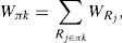

At the beginning it is necessary to group regions into a defined number of partitions (p), so that weights of these partitions are approximately the same, but never greater than the maximal partition weight M defined as:

where W_πk is partition weight, p is the number of partitions, and ε ∈ [0, (p-1)/p] is the tolerance.

The optimization criterion should obtain the maximum connection inside a partition:

where function φ_k is given by Eq. 2, and all partition weights are constrained by:

Based on these defined optimization criteria, graph partition algorithms are applied. The result of the algorithm is a division of data (grouped into the roots) by partitions (processors). Assuming that the task is to divide the distributed network (shown in Figure 1) into three partitions with tolerance ε = 0.1 (M = 32.27), the result would be partitioning (as in Figure 3):

Figure 1.

An example of initial data model in power distribution system [17].

3

PSO algorithm

PSO algorithm is a stochastic optimization technique based on the collective intelligence of the population. Kennedy and Eberhart [18], inspired by the behaviour of a flock of birds looking for food [19], developed PSO algorithm which follows common behaviour features of animals that move in groups. A population, the so called swarm, consists of particles which move through multidimensional space and change their positions, depending on their own experience and the experience of the other particles. At first, the algorithm was developed for continual systems, and later - algorithms for discrete systems were introduced: binary PSO [20] and integer PSO [21-23]. With the binary algorithm each particle from the population can take binary values (0 or 1). In more general cases, such as integer PSO, an optimal value is achieved by rounding the real optimum to the nearest integer.

Particle representation. Supposing the given graph G=(V,E) with a set of vertices (roots) V={v₁, v₂,…, v_d} should be divided into p partitions. In that case, the solution is represented by the vector of d elements, the values of which are indices of the given partitions (integer between 1 and p) [23, 24].

For example, for a graph with 8 vertices, which is divided into 3 partitions, the solution 12332131 refers to the following:

By adapting PSO algorithm to the graph partitioning problem, the dimension of particles is equal to the number of vertices in the graph. Particle positions are updated in a defined number of iteration, in accordance to optimisation criteria, and the bestparticle position is searched.

The change of particle i position is achieved by moving the particle from the previous position, according to equation:

where:

-xik - position of particle i in iteration k,

vik=1 - velocity of particle i in iteration (k+1).

Updating of velocity Vik=1, for each dimension, is carried out according to:

where:

• -

  W - inertia factor,

• -

  C₁ - individuality factor (constant),

• -

  C₂ - social factor (constant),

• -

  bi−xik – individual component (b_i is the best position for particle i),

• -

  bg−xik – social component (b_g is the best position for all particles),

• -

  r₁ and r₂ random numbers from [0,1].

For the updated position Xik+1, the optimisation criteria F is calculated. Position Xik+1 is memorised as the best for particle i - bi and the population - b_g (if it is better than the previously best position). High velocity of particle movement results in significant position change, so a maximum velocity limit is introduced (v_M):

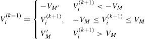
In order to get a versatile velocity for all particle dimension, a further modification of already defined velocity Vik+1 is:

where Δx_maxr is the range for velocity modification (Δx_max is the highest possible change of position, and r is random number r∈(0,1]).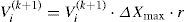

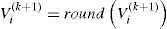
PSO is basically algorithm for solving continual problems. Therefore, it is necessary to adopt PSO to the discrete problem and define the allowed space for particle positioning. First, velocity is rounded to the nearest integer:

Particle position must have integer values from interval (0, p], so at the and a position modification, according to module p, is carried out:

where mod(a,b) - the remainder while dividing a with b (remainder 0 is related to partition ρ).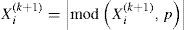

After defined number of iterations, the division of vertices into partitions is achieved as the best particle position in population b_g.

4

Distributed PSO algorithm

Distributed PSO algorithm is based on parallel space searching for available solutions [25]. The population (swarm) consists of several distributed sub-swarms, alocated to different processors (shown in figure 4).

Figure 4.

Distributed PSO algorithm (system architecture).

Indipendently of the remaining sub-swarms, the algorithm (a defined number of iterations) is executed on local sub-swarms by each processor. After a formerly defined number of iterations, solutions of different sub-swarms are exchanged. Modification in the distributed algorithm is the introduction of a new parameter – synchonisation period (T_sync), which defines the frequency of communication between sub-swarms. Parameter T_sync represents the number of iterations afer which the global optimum (b_g) will be updated. When sub-swarms receive information about global optimum they change velocity as shown in Eqs. 7-10.

The way of algorithm execution is changed by synchronisation period modification. In case of low T_sync values, sub-swarms are more independent and the parallelisation effect is less stressed. In additionto that, the algorithm is slower due to the communication between sub-swarms. On the other hand, sub-swarms are more independent for higher values of synchronisation period, but this can affect the quality of solution.

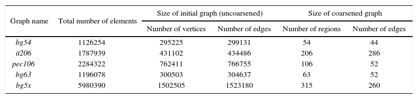
5

Experimental results

We tested the models of the real electric power distribution network. The network characteristics are shown in Table 1.

Table 1.

Test data models.

Graph name	Total number of elements	Size of initial graph (uncoarsened)		Size of coarsened graph
		Number of vertices	Number of edges	Number of regions	Number of edges
bg54	1126254	295225	299131	54	44
it206	1787939	431102	434486	206	286
pec106	2284322	762411	766755	106	52
bg63	1196078	300503	304637	63	52
bg5x	5980390	1502505	1523180	315	260

Models bg54 and bg63 are different versions of Belgrade (Serbia) power distribution network. Pec106 is a part of North Carolina (United States) power distribution network model; it206 is a network model of Milano (Italy); and bg5x is Belgrade network model multiplied five times.

5.1

PSO algorithm

PSO algorithm is tested for following parameters:

• -

  number of particles - depends on size of graph:

  • -

    bg54 and bg63 - 100 particles,

  • -

    pec106 - 110 particles,

  • -

    it106 - 220 particles, and

  • -

    bg5x - 330 particles.

• -

  inertia W is set on 0.9 and linearly decreases up to 0.4 for previously given number of iterations (recommendation from[24]),

• -

  velocity v is limited by total number of partition v ≤ |V_max| ≤ ρ.

• -

  C1 = C₂ = 2.

• -

  tolerance ε ∈ {0.1, 0.2, 0.3}

• -

  maximal number of iterations - maxIt =5000

• -

  number of repetitions for each test - 100 times.

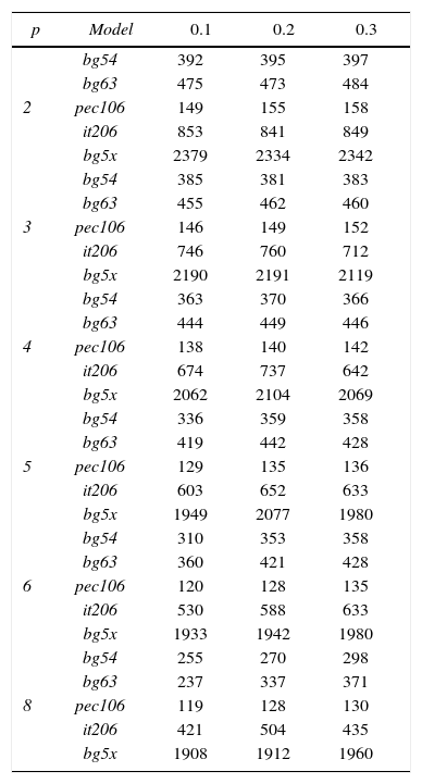
Results representing average values for 100 tests are shown in the table 2.

Table 2.

PSO algorithm results.

p	Model	0.1	0.2	0.3
2	bg54	392	395	397
	bg63	475	473	484
	pec106	149	155	158
	it206	853	841	849
	bg5x	2379	2334	2342
3	bg54	385	381	383
	bg63	455	462	460
	pec106	146	149	152
	it206	746	760	712
	bg5x	2190	2191	2119
4	bg54	363	370	366
	bg63	444	449	446
	pec106	138	140	142
	it206	674	737	642
	bg5x	2062	2104	2069
5	bg54	336	359	358
	bg63	419	442	428
	pec106	129	135	136
	it206	603	652	633
	bg5x	1949	2077	1980
6	bg54	310	353	358
	bg63	360	421	428
	pec106	120	128	135
	it206	530	588	633
	bg5x	1933	1942	1980
8	bg54	255	270	298
	bg63	237	337	371
	pec106	119	128	130
	it206	421	504	435
	bg5x	1908	1912	1960

5.2

Distributed PSO algorithm

Distributed PSO (DPSO) algorithm is implemented in C# programming languege, and swarm clusterisation is done on Windows HPC Server 2008 operative system. For communication between sub-swarms MPI (Message Passing Interface) [26, 27] communication protocol is used.

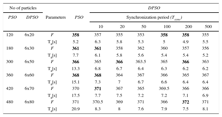
A comparison of classic (sequential) PSO and DPSO algorithm on model bg63 is carried out with following parameters:: W = [0.9, 0.4], C₁ = 2, C₂ = 2, particle dimension is 63, maxIt = 1000,ε = 0.1, ρ = 6. The testing of distributed algorithm is done on 6 sub-swarms, on 6 processors. Execution time T_a and the value of the optimisation function F are analysed for the same number of particles in both algorithms (but the swarms in the DPSO are divided into 6 sub-swarms).

Test results for sequential and distributed algorithm are shown in the table 3. The results represent average values for 100 repetitions of tests. Tests were carried out for different population sizes (120-480 particles) and for varying synchronization time in DPSO algorithm: T_sync ∈ {10, 20, 50, 100, 200, 500}.

Table 3.

Sequential (PSO) and distributed PSO (DPSO) algorithms results for 100 iterations.

No of particles		Parameters	PSO	DPSO
PSO	DPSO			Synchronization period (Tsync)
				10	20	50	100	200	500
120	6x20	F	358	357	355	353	358	358	355
		Ta[s]	5.2	6.3	5.8	5.3	5	4.9	5.5
180	6x30	F	361	361	358	362	360	357	356
		Ta[s]	7.7	6.1	5.8	5.6	5.4	5.4	5.2
300	6x50	F	366	365	366	363.5	365	366	363
		Ta[s]	13.3	6.8	6.7	6.4	6.3	6.2	6.2
360	6x60	F	368	368	364	367	366	365	367
		Ta[s]	15.1	7.3	7	6.7	6.6	6.4	6.4
420	6x70	F	370	371	367	365	369.5	366	366
		Ta[s]	17.5	7.7	7.5	7.2	7.2	7.1	6.9
480	6x80	F	371	370.5	369	371	366	372	371
		Ta[s]	20.9	8.3	8	7.6	7.9	7.5	8.1

Execution times of sequential PSO and DPSO algorithms (for varying synchronization time) are shown in Figure 5.

Figure 5.

Execution time of sequential and distributed PSO (for different T_sync).

Based on these results the following can be concluded:

• 1.

  Execution time of DPSO reduces with increasing synchronization time (T_sync),

• 2.

  If the population size is 300 or more particles - execution time of DPSO is significantly less (2 times or more) than execution time of PSO,

• 3.

  When the population is small - frequent communication (lower value of T_sync) between sub-swarms is required in order to achieve the same results as a sequential algorithm,

• 4.

  If the number of particles in sub-swarms is not less than the size of the particle, DPSO gives better results for the criterion function F and significantly shorter execution time,

• 5.

  The execution time of DPSO with a population 6x80 particles is comparable to the execution time of the sequential PSO algorithm (with population of 180 particles), and much better results are achieved (372/361) by DPSO,

• 6.

  Using DPSO algorithm is recommended in case of larger graphs. If the size of the particle is greater than 300 (i.e., if the graphs have more than 300 vertices), then the use of parallel DPSO algorithm is reasonable.

6

Conclusion

The paper presents a method for partitioning a data model of the power distribution network in order to optimize the analytical power calculations. The classical PSO (sequential) and distributed PSO algorithm are applied, and experiments are performed in the distributed multiprocessor system. Experiments showed that the distributed PSO algorithm achieved better results than the sequential PSO algorithm.