Materials Supply System Analysis Under Simulation Scenarios in a Lean Manufacturing Environment

Abstract

Identifying the most efficient supply system for a company working under Lean Manufacturing practices was possible with the support of this work. Promodel software was used to develop simulation model depicting a constant velocity joints (CVJ) production system, where two different supply methods were assessed. According to results herein obtained, better performance is achieved under random supply method in comparison with a clustering supply method. The company’s goal is to keep 1% losses due to lack of material. In the actual process, this essential parameter was reduced from 2.73% to 1.177%, if random supply method is properly implemented.

1

Introduction

Supply chain management involves the coordination of several areas such as production, warehouse, location and transportation among its members to achieve the best combination of response capacity and efficiency to the market it supplies. There are five areas over which the company can take defining decisions regarding its supply chain capacity, such as production, warehouse, location, transportation and information [1]. This paper will focus on warehouse and production, in the specific case of a constant-velocity joints (CVJ) manufacturing company.

The key strategy of supply chain is to be efficient throughout the chain, and in order to achieve this goal many worldwide companies are adopting Lean Manufacturing production practices, which lead to a better competitive position [2]. After the benefits obtained when implementing these practices, an evident problem arise such as losses due to a lack of material.

Excess of raw material inventories and work in process are a major concern for an efficient supply chain, and to mitigate their impact flow tools such as pull system, SMED (single-minute exchange of died), balanced production, groups’ technology, etc, are applied. However, in the extent the model changes and process are decreased, the continuity of cells is in risk due to lack of materials [3].

To counteract this effect, this work proposes to assess two supply methods in a Lean Manufacturing-based company, performed with the support of an outstanding too called Discrete-Event Simulation (DES).

Due to the nature of the company it is not possible to modify actual facilities, since the company is classified as tier one within the automotive industry, i.e., it delivers the products directly to several car manufacturers’ plants such as VW, Ford, Nissan, Honda, GM, etc. To increase the rate for success in a Lean Manufacturing project, Standridge stands that a convenient alternative is to apply simulation [4]. It has been shown that the simulation can be applied to the analysis of supply chains [5]. This paper proposes the use of the simulation using Promodel software, giving flexibility to make experiments without using actual systems. Two scenarios were executed in this model. In the first one, the possibility of supplying the materials from the warehouses to the production cells with a clustering approach is assessed, e.g., each forklift operator (router) can only deliver to the cells he was assigned to. To cluster, the hierarchical clustering analysis (HCA) was used [6]. In the second scenario, any router can take materials from any warehouse and deliver them to the production cell that requires it.

Since the strategy of clustering has shown to give good results, a logistical problem of delivery and picking up of packages had been addressed, by applying a strategy of sectorization, similar to the one called cluster in our work [7]. Our proposal compares the delivery and collection of materials using cluster against random deliveries.

The rest of the paper is structured as follows: section 2 defines the methodology; in section 3, the production system operation is described; section 4 explains the materials supply system; in section 5, the proposed supply systems are defined; in section 6 the steps to build the simulation model are listed; in section 7 the results of both scenarios are shown; and in section 8, conclusions are given.

2

Materials and methods

2.1

Description of the current production system

It is very important to understand the current production system to define correctly the problem.

2.2

Description of the supply system

In the production system, there is a supply chain system, that provides materials to the cells production.

2.3

Simulation model

It is a platform that let us analyze the supply system in different scenarios. Seven steps were followed and will be described in section 6.

2.4

Recommendations

After running the simulation model, it is possible to give recommendations based on the results.

3

Production system description

The manufacturing plant where this project was developed produces constant-velocity joints (CVJ), fundamental means of transmitting power from the differential to the wheels. The production system has 20 cells but only 17 are considered because of the demand of work; each one produces a family of products for different car manufacturers such as Ford, Renault, Hyundai, VW, GM, etc. The production quantities, the model and sequence in which they will be produced are recorded in the heijunka box. This can be translated as production leveling or smoothing and within Lean Manufacturing practices, it suggests to process small product lots on a frequent basis [8].

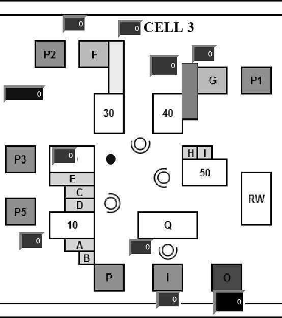
Figure 1 shows the cell 3; every cell has the same configuration. Each cell counts with 4 operators who are responsible for the assembly of each one of the components up to final product. They take all parts that compose the product from a location called usage point. A resource called supplier boy, who puts each component in the usage point, avoids the operators from moving in search of components.

Figure 1.

Cell 3.

The finished goods are stored in racks called plastics, which purpose is to protect the finished goods. Once the amount of scheduled parts indicated in the heijunka box is completed, a model change is performed to begin the manufacturing of the next scheduled product lot.

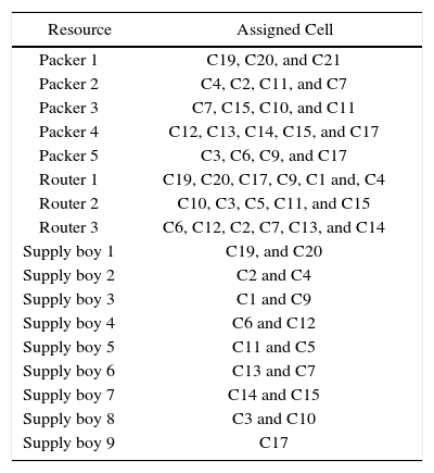
4

Supply systems description

Wishing to process small product lots and in order to keep the parameter work in process (WIP) at a minimum level a new supply system was implemented. To fulfill the goal, a supply strategy was established, where materials are delivered just after the manufacturing of any model is completed in the cell and the model change is triggered [3]. The materials handling system is composed by the following resources: 5 packers, 3 routers (forklift operators) and 9 supply boys assigned as seen on Table 1. In a simulation approach a resource means a person or equipment used to transport raw material or finished good [9].

Table 1.

Resources.

Resource	Assigned Cell
Packer 1	C19, C20, and C21
Packer 2	C4, C2, C11, and C7
Packer 3	C7, C15, C10, and C11
Packer 4	C12, C13, C14, C15, and C17
Packer 5	C3, C6, C9, and C17
Router 1	C19, C20, C17, C9, C1 and, C4
Router 2	C10, C3, C5, C11, and C15
Router 3	C6, C12, C2, C7, C13, and C14
Supply boy 1	C19, and C20
Supply boy 2	C2 and C4
Supply boy 3	C1 and C9
Supply boy 4	C6 and C12
Supply boy 5	C11 and C5
Supply boy 6	C13 and C7
Supply boy 7	C14 and C15
Supply boy 8	C3 and C10
Supply boy 9	C17

The 3 routers are responsible for taking materials from machined and plastics warehouse and move them towards the production cell that has been assigned, just at the moment of model change for producing the next scheduled product, with the purpose of having all materials available at the required time and thus to reduce WIP at minimum value.

The packers are responsible for assembling the packs according to the scheduled amounts of each model in the heijunka boxes on production cells. The packs are composed by diverse materials (miscellaneous), which are parts like dampers, ties, locks, etc. For example, if a 240 piece lot is scheduled for model x, the packer has to prepare the pack of miscellaneous composed by 480 boots, 240 locks, 240 dampers, 240 ties, etc.

The supply boys attend two adjacent cells. Their role is to take materials that have been moved by routers and packers and to put them in the location called usage point within the production cells, and from there operators take the parts and execute the corresponding assembly. This way the supply boys do not need to move from the cells to the warehouse. This helps to avoid wasting great amount of time due to unnecessary movements and it allows the supply boy to attend up to two production cells [10].

5

Supply based on clusters vs random supply

The way materials are supplied according to the system is defined in Table 1. Such system was empirically designed, based on expertise from staff members like supervisors, routers (forklift operators) and storekeepers. As it can be noted, the scarcest resources are routers. They are responsible for lack of materials on production cells, therefore the analysis will focus on them and improvements will be defined considering the opportunity to make modifications in the routers’ operation. With regards to supply boys and packers, there will not be any modifications on their conditions.

5.1

Supply based on cluster

Cluster is the classification of data in groups with similar features. The issue of clustering has been approached in many situations by researchers in several sciences, and makes this tool very useful and easy to apply. Clustering is sometimes difficult to develop due to its combinatorial complexity. Jain performed deep analysis of cluster techniques [6].

Given the supply system characteristics, applying the hierarchical clustering analysis (HCA) is here proposed, the HCA being usually used when the exact number of clusters is required and few elements are available. In this case, there will only be three clusters, since there are only three routers to whom assign the different production cells that they will attend.

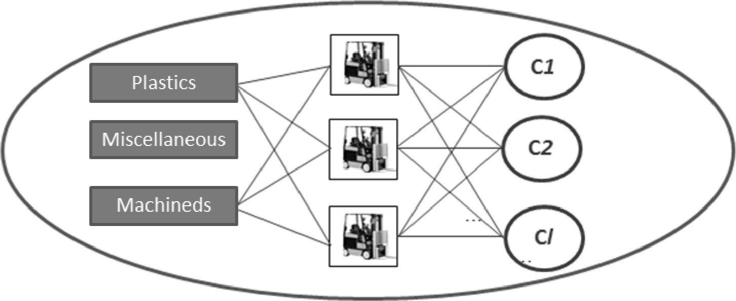
5.2

Random supply

Figure 2 shows the architecture proposed for random supply. It can be detected that routers are able to load materials from plastics and machined warehouse and deliver them to the production cell as may be required.

Figure 2.

Architecture of random supply system.

This means that any router can take materials from the plastics or machined warehouse and deliver them to the production cell that requires it, and are not restricted to supply only to any given production cell. The performance is assessed in the simulation model.

6

Simulation model

Due to the complexity of analyzing the system herein described, it is recommended to use simulation. This tool has proven to be successfully applied to projects related to Lean Manufacturing practices, like Standridge concludes in his research [4]. The simulation model was built following a methodology of seven steps that will be outlined below [9].

6.1

Problem definition

It is one of the most important steps since if from the beginning the project is properly defined, the solution is obtained in great extent. The goal is to reduce the losses (waiting) by lack of supply the production cells are subjected to when they are not supplied in time, once the changeover is completed.

6.2

Data acquisition and analysis

This stage consists in collecting data and defining the probability distribution they follow through goodness-of-fit tests. The most important data for building the model were the following: router speed, distances from warehouse to different production cells, each cell’s cycle time, model changes duration and losses by lack of material. However, per request of the company and its protection, the detail of this step is not shown.

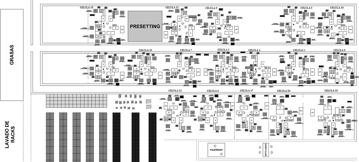
6.3

Model design

The simulation model was developed using Promodel software and its huge capacity to depict discrete manufacturing systems. Figure 3 shows the developed model layout.

Figure 3.

Plant layout model developed with Promodel.

6.4

Verification and validation

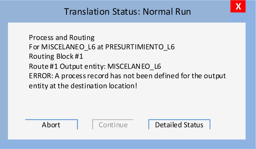
Before taking any decision based on results coming from the simulation model, it is fundamental that the developed model exactly represents the actual system [9]. First, the verification must be made in order to assure the model behaves as expected. Then validation is performed, which consists in defining if the simulation model behaves just like the actual system. For the verification, the model was developed in stages, i.e, elements were progressively added and the model executed without being finished at all. This was made with the purpose of detecting errors using the embedded debugging tool of the software. Figure 4 shows a message box from the debug tool. The message indicates that the “miscelaneo” that would be sent to cell 6 has not yet declared the target location; therefore it is not able to find its output.

Figure 4.

Software debugger tool to verify model.

Validation was performed using two techniques suggested by Harrell and Sargent: visual validation and by comparison of historical records [10, 11]. The first technique implies running the simulation process and to monitor the movements of resources such as packers, supply-boys and routers. It was also validated that cells started assemblies once they have materials like machined, miscellaneous, and plastics. After it was detected that all movements performed in the actual system are also included in the model, it was considered as validated by the visualization technique.

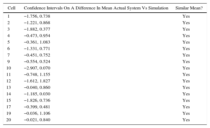
The second validation technique applied was comparison of historical records from actual system against data coming from the simulation model. Losses by lack of materials was the most important parameter, therefore it was analyzed in this study. Historical records were taken over the last eight months. As such, enough data could be gathered since 20 data can be collected every month. To validate the results of the simulation model, we used a 95% confidence intervals on a difference in mean to define if average losses by lack of materials in the real system is equal with the results of the simulation model, using equation (1) [12]:

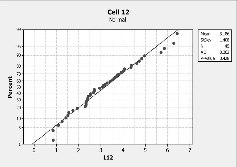
We assume that the sample means and variances are from two independent normal populations. We did a goodness-of-fit test to ensure that the data follow a normal distribution. Figure 5 shows an example with cell 12. Every set of data was tested in order to validate the normality.

Figure 5.

Goodness-of-fit normality in data of cell 12.

Results from the simulation model and historical data from current system were considered as well as 95% confidence interval on a difference in means for the losses due to lack of material coming from the simulation model and current system. The confidence intervals are listed on Table 2, where only 17 cells currently working according with the demand appear.

Table 2.

Model validation.

Cell	Confidence Intervals On A Difference In Mean Actual System Vs Simulation	Similar Mean?
1	−1.756, 0.738	Yes
2	−1.221, 0.868	Yes
3	−1.882, 0.377	Yes
4	−0.473, 0.954	Yes
5	−0.361, 1.083	Yes
6	−1.331, 0.771	Yes
7	−0.451, 0.752	Yes
9	−0.554, 0.524	Yes
10	−2.907, 0.070	Yes
11	−0.748, 1.155	Yes
12	−1.612, 1.827	Yes
13	−0.040, 0.860	Yes
14	−1.185, 0.030	Yes
15	−1.826, 0.736	Yes
17	−0.399, 0.481	Yes
19	−0.036, 1.106	Yes
20	−0.021, 0.840	Yes

If the confidence interval includes zero, it implies that the means are equals [12]. In the results listed in Table 2, it can be detected that every confidence interval includes zero; therefore, the means of the simulation model and actual system are equal and that the simulation model is statistically considered valid and can be used as a tool to perform the experiment.

6.5

Warm up determination

In a simulation model, it is important to define the time at which steady state conditions are met [13]. The statistical information collected during the warm-up stage is not considered for analysis, and therefore Promodel software discards the information created during such period. The simulation starts when the system is empty, which is not a steady state condition. This can only be achieved when all manufacturing cells had started at least their first scheduled production lot. Taking this into consideration, a variable which counts from zero was implemented to the model, “zero” meaning that no cell has started to operate, up to 17, meaning that all production cells had started to process at least their first scheduled lot. 15 repetitions were executed to define the time at which a steady state is achieved and it was found that in each repetition, the variable reaches the value of 17 after 4 hours. This allowed defining a warm-up period of 4 hours.

6.6

Experimental

Two experiments were performed. In the first one the model was programmed considering the clusters defined in Figure 7. In the second experiment the model was programmed under random supply design, in which the restriction for routers to deliver only to its assigned cluster was removed.

Figure 6.

Plant layout.

Figure 7.

Clusters obtained with Minitab.

6.7

Results analysis

The results are described in detail in the following section.

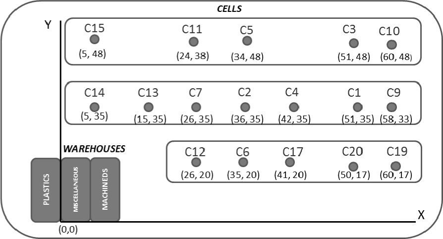
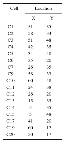
7

Results

To define clusters based on HCA, the distances from each production cell regarding the warehouse were defined, marked with position (0, 0) as can be seen in Figure 6, where the distances are in meters. The distances were considered quadratic, because of the limits of the configuration.

Considering distances shown in Figure 6, it is possible to define the location of cells in a Cartesian plane in the first quadrant and then record their X and Y values, which are listed in Table 3.

Table 3.

Cells location.

Cell	Location
	X	Y
C1	51	35
C2	58	33
C3	51	48
C4	42	35
C5	34	48
C6	35	20
C7	26	35
C9	58	33
C10	60	48
C11	24	38
C12	26	20
C13	15	35
C14	5	35
C15	5	48
C17	41	20
C19	60	17
C20	50	17

The information in Table 3 was collected with Minitab statistical software, to define clusters using the following steps: Stat – Multivariate – Cluster Observations – Variables or distance matrix – Link method (Average) - Distance measure (Squared) – Number of cluster (3) – Show dendogram – customize – Title (Clusters) - Case labels (Cells) – Label Y axis with (Distance) – Show dendogram in (One Graph) – ok.

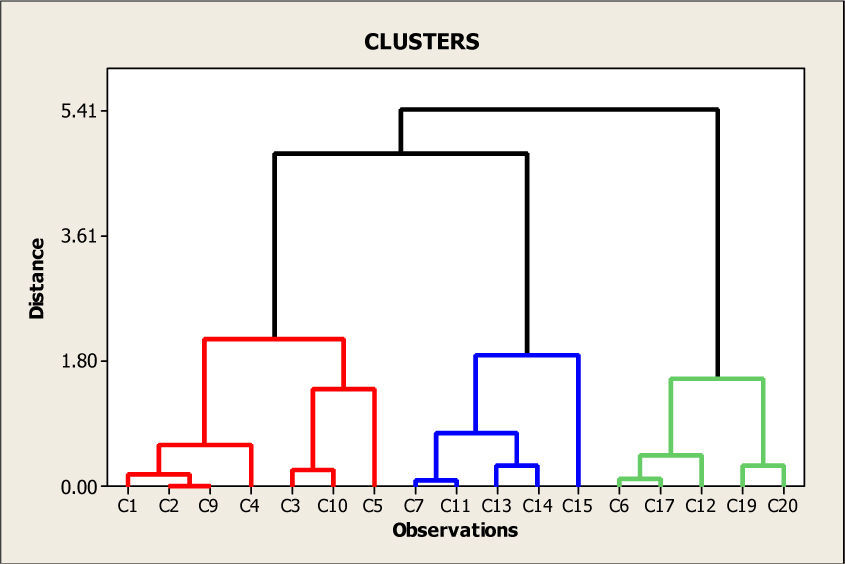
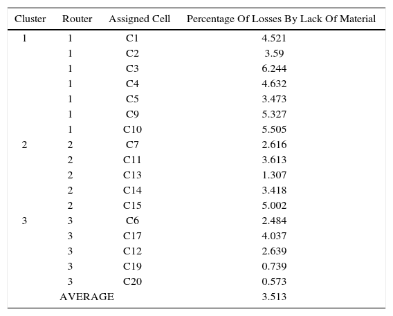
After completing the steps previously mentioned, the final clustering is clearly seen in Figure 7. This clustering suggests that Router 1 supplies C1, C2, C3, C4, C5, C9, and C10 cells (in red). The router 2 supplies C7, C11, C13, C14, and C15 cells (in blue); and finally, the router 3 supplies C6, C12, C17, C19 and C20 cells (in green).

This proposal will be analyzed on the simulation model to calculate its performance before implementing it to the actual system. Each repetition was executed during 24 hours, since statistics obtained from actual system were obtained considering this period of time. The following table lists the results when routers supply materials by HCA clustering. Using the tool Stat:fit, it was defined that for a 95% confidence level and 1% of maximum allowed error, 50 repetitions were required. The average results are listed in Table 4.

Table 4.

Losses by lack of material for current clusters and random supply systems.

Cluster	Router	Assigned Cell	Percentage Of Losses By Lack Of Material
1	1	C1	4.521
	1	C2	3.59
	1	C3	6.244
	1	C4	4.632
	1	C5	3.473
	1	C9	5.327
	1	C10	5.505
2	2	C7	2.616
	2	C11	3.613
	2	C13	1.307
	2	C14	3.418
	2	C15	5.002
3	3	C6	2.484
	3	C17	4.037
	3	C12	2.639
	3	C19	0.739
	3	C20	0.573
AVERAGE			3.513

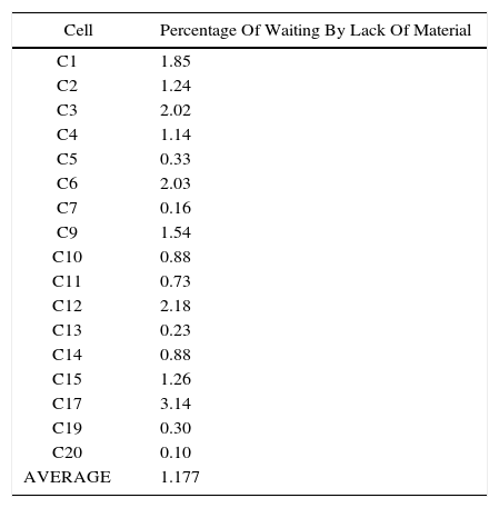
For the random supply scenario and also considering a 95% confidence level and 1% of maximum allowed error, it was defined that for proper average calculation, executing 45 repetitions was required. The results are listed in table 5.

Table 5.

Losses by lack of material under random scenario.

Cell	Percentage Of Waiting By Lack Of Material
C1	1.85
C2	1.24
C3	2.02
C4	1.14
C5	0.33
C6	2.03
C7	0.16
C9	1.54
C10	0.88
C11	0.73
C12	2.18
C13	0.23
C14	0.88
C15	1.26
C17	3.14
C19	0.30
C20	0.10
AVERAGE	1.177

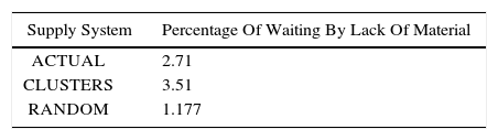
Table 6 lists a summary with results, where the average system performance for each scenario can be seen.

Table 6.

Losses by lack of material for current, clusters and random supply systems.

Supply System	Percentage Of Waiting By Lack Of Material
ACTUAL	2.71
CLUSTERS	3.51
RANDOM	1.177

8

Conclusions

Three different scenarios were studied, current supply system, supply system using clusters defined by HCA method and random supply method. According to the results listed in Table 6 from the previous section, it is recommended to use the random supply method, taking into account that the goal is to reduce losses by lack of material.

The random supply system is very complex, since any router (the first that is available) can take materials from any warehouse (plastics or machined) and deliver them to the production cell that is making its request. To decrease complexity, it is recommended to combine the system with an Andon system, which has visual and audio elements helping to inform about downtimes under certain circumstances. In this case, a blue color is suggested to point out that materials are required since most authors suggest the blue color for the lack of material.

The Andon system should be synchronized to bond the cell needs with the first available router since it was able to implement it in the simulation process. However, to apply it in the actual system would be hard to accomplish, but not impossible.

To make the final decision, several criteria must be considered. For example, if clustering supply method is used, the materials supply management is made easier, in great extent due to the fact that every router knows in advance the cells that will be supplied, but it faces losses by lack of materials.

On the other hand, if random supply is selected, the milestone will be that different routers deliver at the exact moment to the production cells, i.e, when they need it.

Using this proposal, it makes it easier to apply flow tools related to Lean Manufacturing, like small production lots, to make frequent model changes, balanced production, WIP reduction, etc., since materials will be delivered at the moment they are required.

An important restriction for applying this solution is that company’s production must be performed under Lean Manufacturing practices. Besides, it is required that staff is capable to make simulations, in order to first analyze the supply of materials in the simulation model.

In the three supply systems; actual, clustering and random, the routers can only take one load and deliver it to its location (from the warehouse to the cells for the case of raw materials or from the production cell to safe launch area in the case of finished Goods). Therefore it is recommended to analyze scenarios where the possibility for routers to deliver more than one load and make materials deliveries in one single trip, performing loads and unloads, delivering raw materials and taking finished goods is considered. For further research, modifying the company’s supply system is proposed, to apply the mentioned restrictions in the vehicle router problem (VRP) where more than one load can be taken and in a single trip load and unload materials, without the need of returning to the warehouse.

Acknowledgments

This project was performed thanks to support given by Conacyt through scholarship No. 228973 for funding my specialization studies and we wish to thank CIATEC, where training about industrial engineering topics were given by expert personal.