This paper presents three approaches dealing with the feedback control of nonlinear analytic systems. The first one treats the optimal control resolution for a control-affine nonlinear system using the State Dependant Riccati Equation (SDRE) method. It aims to solve a nonlinear optimal control problem through a Riccati equation that depends on the state. The second approach treats a procedure of constructing an analytic expression of a nonlinear state feedback solution of an optimal regulation problem with the help of Kronecker tensor notations. The third one deals with the global asymptotic stabilization of the nonlinear polynomial systems. The designed state feedback control law stabilizes quadratically the studied systems. Our main contribution in this paper is to carry out a stability analysis for this kind of systems and to develop new sufficient conditions of stability. A numerical-simulation-based comparison of the three methods is finally performed.
The optimal control of nonlinear systems is one of the most challenging and difficult topics in control theory. It is well known that the classical optimal control problems can be characterized in terms of Hamilton-Jacobi Equations (HJE) [1, 2, 3, 4, 5, 6]. The solution to the HJE gives the optimal performance value function and determines an optimal control under some smooth assumptions, but in most cases it is impossible to solve it analytically. However, and despite recent advances, many unresolved problems are steel subsisting, so that practitioners often complain about the inapplicability of contemporary theories. For example, most of the developed techniques have very limited applicability because of the strong conditions imposed on the system [29, 40, 41, 42, 43]. This has led to many methods being proposed in the literature for ways to obtain a suboptimal feedback control for general nonlinear dynamical systems.
The State Dependent Riccati Equation (SDRE) controller design is widely studied in the literature as a practical approach for nonlinear control problems. This method was first proposed by Pearson in [7] and later expanded by Wernli and Cook in [8]. It was also independently studied by Cloutier and all in [9, 31, 34]. This approach provides a very effective algorithm for synthesizing nonlinear optimal feedback control which is closely related to the classical linear quadratic regulator. The SDRE control algorithm relies on the solution of a continuous-time Riccati equation at each time update. In fact, its strategy is based on representing a nonlinear system dynamics in a way to resemble linear structure having state-dependant coefficient (SDC) matrices, and minimizing a nonlinear performance index having a quadratic-like structure [9, 24, 34, 35, 38]. This makes the equation much more difficult to solve. An algebraic Riccati equation using the SDC matrices is then solved on-line to give the suboptimum control law. The coefficients of this equation vary with the given point in state space. The algorithm thus involves solving, at a given point in state space, an algebraic state-dependant Riccati equation, or SDRE.
Although the stability of the resulting closed loop system has not yet been proved theoretically for all system kinds, simulation studies have shown that the method can often lead to suitable control laws. Due to its computational simplicity and its satisfactory simulation/experimental results, SDRE optimal control technique becomes an attractive control approach for a class of non linear systems. A wide variety of nonlinear control applications using the SDRE techniques are exposed in literature. These include a double inverted pendulum in real time [26], robotics [12], ducted fan control [37, 38], the problems of optimal flight trajectory for aircraft and space vehicles [22, 30, 32, 36] and even biological systems [10, 11].
An other efficient method to obtain suboptimal feedback control for nonlinear dynamic systems was firstly proposed by Rotella [33]. A useful notation was developed, based on Kronecker product properties which allows algebraic manipulations in a general form of nonlinear systems. To employ this notation, we assume that the studied nonlinear system is described by an analytical state space equation in order to be transformed in a polynomial modeling with expansion approximation. In recent years, there have been many studies in the field of polynomial systems especially to describe the dynamical behavior of a large set of processes as electrical machines, power systems and robot manipulators [14, 15, 16, 17, 18]. A lot of work on nonlinear polynomial systems have considered the global and local asymptotic stability study, and many sufficient conditions are defined and developed in this way [14, 15, 19, 20, 21, 39].
The present paper focuses on the description and the comparison of three nonlinear regulators for solving nonlinear feedback control problems: the SDRE technique, an optimal regulation problem for analytic nonlinear systems (presented for the first time by Rotella in [33]) and a quadratic stability control approach. A stability analysis study is as well carried out and new stability sufficient conditions are developed.
The rest of the paper is organized as follows: the second part is reserved to the description of the studied systems and the formulation of the nonlinear optimal control problem. Then, the third part is devoted to the presentation of approaches of the optimal control resolution and quadratic stability control approach, as well as to the illustration of sufficient conditions for the existence of solutions to the nonlinear optimal control problem, in particular by SDRE feedback control. In section 4 we give the simulation results for the comparison of the three feedback control techniques. Finally conclusions are drawn.
2Description of the studied systems and problem formulationWe consider an input affine nonlinear continuous system described by the following state space representation:
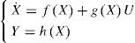
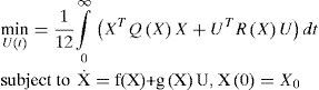
with associated performance index:

where f(X), g(X) and h(X) are nonlinear functions of the state X ∈ Rn, U is the control input and the origin (X=0) is the equilibrium, i.e f(0)=0.
The state and input weighting matrices are assumed state dependant such that: q:rn→rn×n and R:Rn→Rm×m. These design parameters satisfy Q(X)>0 and R(X)>0 for all X.
The problem can now be formulated as a minimization problem associated with the performance index in equation (2):
The solution of this nonlinear optimal control problem is equivalent to solving an associated Hamilton-Jacobi equations (HJE) [1].
For the simpler linear problem, where f(X)=A0X, the optimal feedback control is given by U(X) = −R−1BTPX, with P solving the algebraic Riccati equation PA0+A0TP−PBR−1BTP+Q=0.
The theories for this linear quadratic regulator (LQR) problem have been established for both the finite-dimensional and infinite-dimensional problems [13]. In addition, stable robust algorithms for solving the Riccati equation have been developed and are well documented in many references in literature.
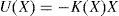
For the nonlinear case, the optimal feedback control is known to be of the form:
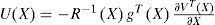
where the function V is the solution to the Hamilton-Jacobi-Bellman equation [1, 3]:

However, the HJB equation is itself very difficult to solve analytically even for the simplest problems. Therefore, efforts have been made to numerically approximate the solution of the HJB equation, or to solve a related problem producing a suboptimal control, or to use some other processes in order to obtain a suitable feedback control. The following section will outline three such methods on feedback control techniques of nonlinear analytic systems.
3Approaches of the feedback control resolution for nonlinear systems formulation3.1SDRE approach to optimal regulation problem formulationThe main problems with existing nonlinear control algorithms can be listed as follows: high computational cost (adaptive control), lack of structure (gain scheduling) and poor applicability (feedback linearization). One method that avoids these problems is the State Dependant Riccati Equation approach. This method, also known as Frozen Riccati Equation approach [28, 29], is discussed in detail by Cloutier, D’souza and Mracek in [35]. It uses extended linearization [27, 31, 35, 8] as the key design concept in formulating the nonlinear optimal control problem. The extended linearization technique, or state dependant coefficient (SDC) parametrization, consists in factorizing a nonlinear system, essentially input affine, into a linear-like structure which contains SDC matrices.
For system (1), under the assumptions f(0) = 0 and for f(.)∈ C1(Rn) [24], we can always find some continuous matrix valued functions A(X) such that it has the following state-dependent linear representation (SDLR):
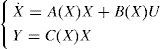
where f(X) = A(X)X and g(X) = B(X), A:Rn →Rn×n is found by mathematical factorization and is, clearly, non unique when n>1, and different choices will result in different controls [25].
The SDRE feedback control provides a similar approach as the algebraic Riccati equation (ARE) for LQR problems, to the nonlinear regulation problem for the input-affine system (1) with cost functional (2). Indeed, once a SDC form has been found, the SDRE approach is reduced to solving a LQR problem at each sampling instant.
To guarantee the existence of such controller, the conditions in the following definitions must be satisfied [25].
Definition 1:A(X) is a controllable (stabilizable) parametrization of the nonlinear system for a given region if [A(X),B(X)] are pointwise controllable (stabilizable) in the linear sense for all X in that region.
Definition 2:A(X) is an observable (detectable) parametrization of the nonlinear system for a given region if [C(X),A(X)] are pointwise observable (detectable) in the linear sense for all X in that region.
When A(X), B(X) and C(X) are analytical functions in state vector X, and given these standing assumptions, the state feedback controller is obtained in the form:
and the state feedback gain for minimizing (2) is:

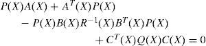
where P(X) is the unique symmetric positive-definite solution of the algecbraic state-dependent Riccati equation (SDRE):
It is important to note that the existence of the optimal control for a particular parametrization of the system is not guaranteed. Furthermore, there may be an infinite number of parameterizations of the system; therefore the choice of parametrization is very important. The other factor which may determine the existence of a solution to the Riccati equation is the selection of the Q(X) and R(X) weighting matrices in the Riccati equation (9).
The greatest advantage of SDRE control is that physical intuition is always present and the designer can directly control the performance by tuning the weighting matrices Q(X) and R(X). In other words, via SDRE, the design flexibility of LQR formulation is directly translated to control the nonlinear systems. Moreover, Q(X) and R(X) are not only allowed to be constant, but can also vary as functions of states. In this way, different modes of behavior can be imposed in different regions of the state-space [26].
3.1.1Stability analysisThe SDRE control produces a closed-loop system matrix ACL(X)=A(X)−B(X)K(X) which is pointwise Hurwitz for all X, in particular for (X=0). Therefore, the origin of the closed-loop system is locally asymptotically stable [9, 24]. However, for a nonlinear system, all eigenvalues of ACL(X) having negative real parts ∀X∈Rn do not guarantee global asymptotic stability [26]. Stability of SDRE systems is still an open issue. Global stability results are presented by Cloutier, D’souza and Mracek in the case where the closed-loop coefficient matrix ACL(X) is assumed to have a special structure [35]. The result is summarized in the following theorem.
Theorem 1:We assume that A(.), B(.), Q(.) and R(.) are C1(Rn) matrix-valued functions, and the respective pairs {A(X), B (X)} and {A(x),Q1/2(X)} are pointwise stabilizable and detectable SDC parameterizations of the nonlinear system (1) for all X. Then, if the closed-loop coefficient matrix ACL(X) is symmetric for all X, the SDRE closed-loop solution is globally asymptotically stable.
Won derived in [3] a SDRE controller for a nonlinear system with a quadratic form cost function presented in the following theorem.
Theorem 2:For the system (1), with the cost function (2), we assume that V satisfies the HJequation (5)and V(X) is a twice continuously differentiable, symmetric and non-negative definite matrix:
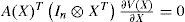
For the nonlinear system given by (1), the optimal controller that minimizes the cost function (2) is given by:
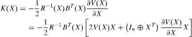
provided that the following conditions are satisfied:
and
where ⊗ is the Kronecker product notation which the definition and properties are detailed in Appendix A.
3.1.2Stability analysis- Main result:We present now our contribution which is the development of sufficient conditions to guarantee the stability of system (6) under cost function (2). Our analysis is based on the direct method of Lyapunov. Firstly, we return to the optimal feedback control (4) and let:
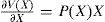
Then the optimal control law can be expressed as:

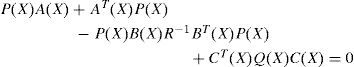
where P(X) is the symmetric positive definite matrix solution of the following State Dependent Riccati Equation :
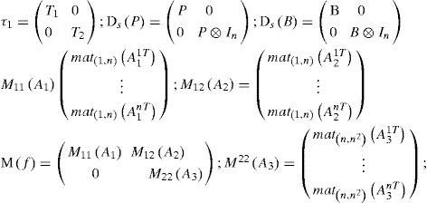
Let us note that such symmetric positive definite matrix P(X) exists, if for any X we have (A(X), M(X), N(X)) is stabilizable detectable, where:
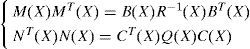
So we assume that this condition is satisfied for each X ∈ R
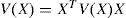
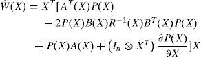
Now let W(X) the Lyapunov function defined by the following quadratic form:
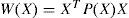
The global asymptotic stability of the equilibrium state (X=0) of system (6) is ensured when the time derivative W˙(X) of W(X) is negative defined for all X ∈ Rn.
One has:

The use of expression (19) and the following equality :
yield :
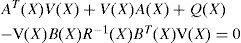
Since AT(X)P(X)−P(X)B(X)R−1BT(X)P(X)+P(X)A(X)=−CT(X)Q(X)C(X) obtained from the SDRE (17), then (22) becomes:
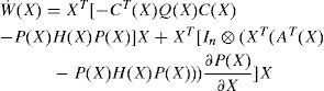
where : H(X) = B(X)R−1(X)BT(X).
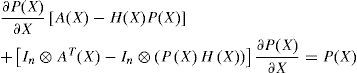
To ensure the asymptotic stability of system (6) with the control law (16), W˙(X) should be negative, which is equivalent to Π(X) negative definite, where:
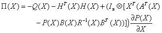
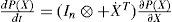
We try now to simplify the manipulation of matrix Π(X) by expressing ∂PX∂X in terms of P(X).
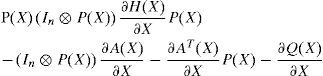
When derivating the SDRE (17) with respect to the state vector X, we obtain the following expression:
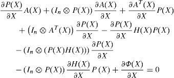
with:Φ(X) = CT(X)Q(X)C(X), which gives:
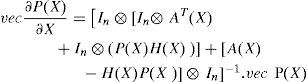
with:
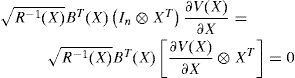
To simplify the partial derivative expression ∂PX∂X, we use ‘vec’ and ‘mat’ functions and their properties defined in Appendix A; then (26) becomes:
which leads to:
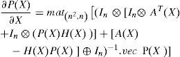
and then we can state the following result:
Theorem 3:The system (6) is globally asymptotically stabilizable by the optimal control law (4), with the cost function (2) if the symmetric matrix Π(X) defined by (24) is negative definite for all X ∈ Rn.
3.2Quasi-Optimal Control for Nonlinear Analytic Cubic SystemWe treat here the procedure presented by Rotella in [33]. It consists in building an analytic expression of a nonlinear state feedback solution of an optimal control problem with the help of tensor notations (57) and (62), detailed in Appendix A. This state feedback will be expressed as a formal power series with respect to X.
Let us consider the system defined by (1), (57) and (62) with an initial condition X(0).
The output function can be expressed by:

where h(.) is a map from Rq into Rp. If h(.) is analytic, it leads to the expression:
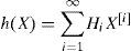
where Hi are constant matrices of adapted dimensions.
The problem of optimal control is to build a state feedback which minimizes the functional cost (2). To find a solution to HJB equation (5), Rotella has proposed in [33] the determination of an analytic form for ∂VX∂X based on the following polynomial expression:
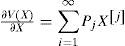
where Pj are constant matrices of adapted dimensions.
In this paper, we consider a nonlinear cubic system defined by:
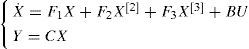
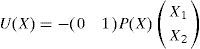
since the truncation of polynomial system, in order three, can be considered being sufficient for nonlinear system modeling. Then the control law of the cubic system (33) can be expressed as:

The determination of the control gains P1, P2 and P3 is deduced from [33]. Therefore P1 is the gain-matrix solution of the optimal control on the linearized system, then P1 is chosen symmetric and solution of the classical Riccati equation:

The second order gain-matrix P2 is expressed as follows:

where:
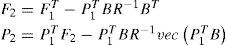
The function ‘vec’ is defined in Appendix A. The third order gain-matrix P3 is given by the resolution of the following expression:
where:
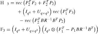
Unfortunately, even if the triplet (F1, B, C) is stabilizable-detectable, the matrix Iq4+Uq×q3 is singular. To overcome this problem, we introduce the notation of the non-redundant i–power X˜;i of the state vector X defined in (52). Then, an analytical function A(X) of X can be written in terms of X[j] as before, and in terms of X˜;j:
Then, by the non-redundant form, (37) must be replaced by the linear equation:
where:
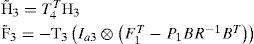
with:
and the matrix T3q is a rectangular matrix of α4 rows and q.α3 columns, which has the property of being of full rank.
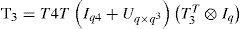
Finally, we obtain the analytical expression of this optimal state feedback:

where:
3.3Quadratic Stabilizing Control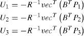
The approach of quadratic stabilizing control exposed in this paragraph was firstly presented in [20]. It consists in the development of algebraic criteria for global stability of analytical nonlinear continuous systems which are described by using Kronecker product. Based on the use of quadratic Lyapunov function, the definition of sufficient conditions for the global asymptotic stability of the system equilibrium was also developed.
We consider the cubic polynomial nonlinear systems defined by the equation (33). Our purpose is to determine a polynomial feedback control law:

where K1, K2 and K3 are constant gain matrices which stabilize asymptotically and globally the equilibrium (X=0) of the considered system.
Applying this control law to the open-loop system (33), one obtains the closed loop system:

Using a quadratic Lyapunov function V(X) and computing the derivative V˙(X) lead to the sufficient condition of the global asymptotic stabilization of the polynomial system, given by the following theorem [20].
Theorem 4:The nonlinear polynomial system defined by theequation (33)is globally asymptotically stabilized by the control law (41) if there exist:
- •
an (n×n) -symmetric-positive definite matrix P,
- •
arbitrary parameters μi,i=1,…,β∈ R
- •
gain matrices K1, K2,K3
such that the η×η) symmetric matrix Q defined by:
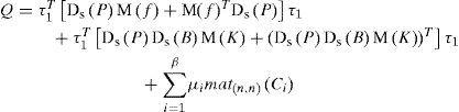
be negative definite where:
with:
- -
Akiis the ith row of the matrix Ak
- -
β = rank(Γ), Γ=Iη2+Uη×ηR+TRT−Iη2
- -
Ci,i=1,…,β are β linearly independent columns of Γ,
- -
µi,i=1,…,βare arbitrary values.
- -
R=τ1+2.U.H.τ2and
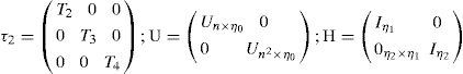
where: η = n1 +n2; η0 =n+ n2; η1 = n2+ n3; η2 = n3+ n4;
In [39], it was proved that the stabilization problem stated by the theorem 4 can be formulated as an LMI feasibility problem.
Theorem 5:The equilibrium (X=0) of the system (42) is globally asymptotically stabilizable if there exist:
- •
a (n×n) -symmetric positive definite matrix P,
- •
arbitrary parameters µi,i=1,…,β ∈ R,
- •
gain matrices K1,K2,K3,
- •
a real γ > 0,
such that
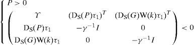
with:
Thus, a stabilizing control law (41) for the considered polynomial system (33) can be characterized by applying the following procedure:
- Solve the LMI feasibility problem i.e. find the matrices
DS(P), W(k) and the parameters and µi and γ such that the inequalities (44) are verified.
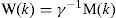
- Extract the gain matrices Ki from the relation M(k) = γ W(k).
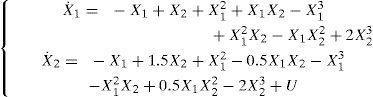
4Simulation resultsIn this section we will compare the performance of the three methods, discussed in the previous paragraph, on a numerical example. We consider a vectorial system defined by the following state equation:
For optimal controls, we focus on minimizing the following criteria:
4.1Application of the SDRE approach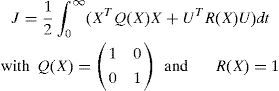
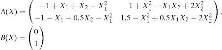
For system (46), we choose the following SDC parametrization:
The controllability matrix is then:
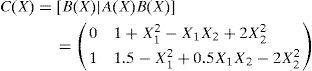
and it has a full order rank for all X, which can justify the good choice of SDC matrices A(X) and B(X).
After solving the state-dependant Riccati equation (9) and obtaining the positive symmetric matrix P(X), the optimal control law can be written as:
We can easily verify that matrix Π(X) given in theorem 3 is negative defined for all X ∈ R, which guarantees the stability of system (46) by the optimal control law (50).
4.2Application of the polynomial approachTo establish the polynomial optimal control law, given by (34), for system (46), we use the procedure of determination of matrices Pi, presented in subsection 3.2. Then we obtain:
4.3Application of the feedback quadratic stabilizing control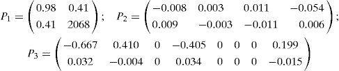
Solving the LMI problem formulated by theorem 5, we obtain:
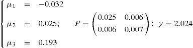
The searched gain matrices, extracted from M(k), are given by:
4.4Numerical simulation
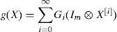
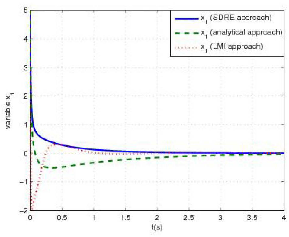
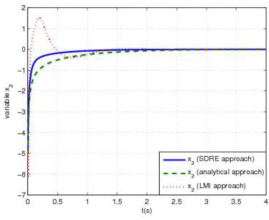
Figure 1 (respectively figure 2) shows the behavior of the first state variable x1(t) (respectively the second state variable x2(t)) of system (46) controlled by the three feedback-control laws illustrated in figure 3. Initial conditions were taken sufficiently far from the origin (x1(0)= − 5, x2(0)=5). Under these conditions, simulations show a satisfactory asymptotic stabilization of state variables for all approaches. Dealing with SDRE technique, simulations lead to the two following direct outcomes:
- •
Stabilization by SDRE approach is almost same or better than other approaches.
- •
For overtaking damping, SDRE technique shows the best results compared to both other approaches with almost no oscillation.


Our main motivation for this contribution was first to expose the main approaches used in the domain of the stability study for non linear systems, then to work on the development of new stability criteria in specific conditions for one technique, and finally to perform a numerical-simulation-based comparison of the three techniques.
The first two approaches are quadratic optimal controls which are determined via the resolution of nonlinear Hamilton-Jacobi equation, where the description of affine-control analytical systems, with Kronecker power of vectors, allows an analytical approximate determination of HJE solution. The third approach is a feedback quadratic stabilizing technique based on the Lyapunov direct method and an algebraic development using Kroneker product properties. Focusing on the first quadratic optimal control approach determined via the resolution of SDRE, our work led to a new result: guarantee the global asymptotic stability of the nonlinear system when some sufficient conditions are verified.
We have then set about some numerical simulations around the three approaches to validate them. One important outcome of these simulations was the proof that SDRE method works better than the analytic ones, which are expected due to the truncation order considered in the polynomial development of the non linear systems. The simulation results have also shown that the SDRE original technique is the easiest to program and to implement.
Further works will consider extension of this synthesis to large scale interconnected nonlinear power systems via decentralized control.
We recall here the useful mathematical notations and properties used in this paper concerning the Kronecker tensor product.
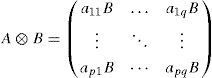
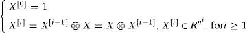
The Kronecker power of order i, X[i], of the vector X ∈ Rn is defined by:
The non-redundant i-power X˜;i of the state vector X = [X1,…,Xq] is defined in [33] as:
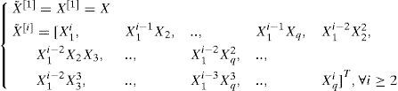
It corresponds to the previous power where the repeated components have been removed. Then, we have the following:
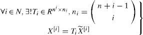
thus, one possible solution for the inversion can be written as:

with Ti+=(TiTTi)−1TiT where Ti+ is the Moore-Penrose inverse of Ti, and ni stands for the binomial coefficients.
Let ein denotes the ith vector of the canonic basis of Rn, the permutation matrix denoted Un×m is defined by [23]:
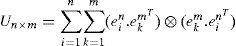
This matrix is square (nm×nm) and has precisely a single “1” in each row and in each column.
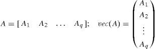

An important matrix valued linear function of a vector, denoted Mat(n,m)(.) was defined in [14] as follows:
If V is a vector of dimension p=n.m then M = Mat(n,m)(V) is the (n×m) matrix verifying: V = Vec(M).
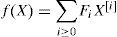
Vector functions : Let f(.) be an analytic function from Rn into Rm. Then f(X) can be developed in a generalized Taylor series using the Kronecher power of the vector X, i.e.
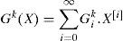
Matrix functions : Let g(.) be an analytic function from Rn into Mn×m(R)(the set of n×m real matrices). Then g(X) can be written as :

where Gk(X) is a vector function from Rn into Rn, which can be written as :
Thus g(X) can be expressed as :
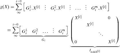
which can be written as: