


The use of short-range wireless for object positioning has seen a growing interest in recent years. This interest is compounded by the inherent GPS limitations especially in indoor situations and in urban canyons. In order to achieve the highest performance of short-range positioning systems it is important to optimize the placement of Base-Stations (BSs) in a given area. The problems of BSs placement to minimize error and to achieve multiple coverage of the area have been addressed separately in the literature. In this paper, we discuss that using short range BSs the two problems are interrelated and need to be solved jointly. We study the impact of different influential attributes of the positioning problem as we alter the layout of BSs in the area. We investigate different scenarios for short-range BSs placement that maximize coverage and minimize positioning error. Simulation results demonstrate that better performance could be achieved using layouts that tend to distribute the BSs uniformly.
We explore the problem of finding the unknown position of an Object of Interest (OoI) in an indoor environment with respect to short-range wireless base stations (BSs). We assume that the BSs are aware of their position and have the ability to exchange this information with the OoI using short-range communication technologies whenever the OoI is within the coverage area of a given BS. The range between the OoI and a BS can be estimated using Received Signal Strength (RSS) [1], Time of Arrival (ToA) [2], Time Difference of Arrival [3], and/or Angle of Arrival (AoA) [4]. Theoretically, once the OoI receives information from three other BSs and the information is error free, it can estimate its position. However, the position information and range estimates are not error free that makes the process of position estimation complicated.
The desire to resolve in-door positioning problems and to complement GPS in problematic out-door situations is generating an increasing interest in the idea of using short-range radios at 2.4GHz, 3.1GHz, 5.9GHz, or 10.6GHz for positioning. Currently, typical approaches use short-range signal based range estimation of the OoI with respect to the BSs. The estimated range values are used to perform tri/multilateration of the OoI position. Information from inertial sensors can also be fused with the range measurements using extended Kalman filter or particle filters [5, 6, 7].
While improved approaches are evolving to enhance range estimation ability, we believe the positioning problem involves more than just ranging. The precision of the estimated position is strongly dependent on the relative geometry of the OoI and the BSs [8]. Therefore, we need to place the BSs in such a way that the position error is minimized. Another coupled problem is the need of higher level of signal coverage throughout the space with a guaranteed availability of multiple signals at every point.
We compare different placement scenarios. We use maintaining the signal coverage, minimizing the Geometric Dilution of Precision (GDoP) and hence maximizing positioning accuracy as our evaluation criteria. We estimate the position of the OoI in a rectangular area with respect to short range BSs. We assume that the OoI and the BSs exist in single plane (2D). This assumption matches most realistic scenarios and reduces the complexity of the localization problem from 3D to 2D. In our application environment, the OoI can move to any point in the area, therefore the performance of the position estimation algorithm needs to be evaluated over the entire area. The BSs employ short-range wireless and the signal of each BS is limited to a fixed circular range assuming omnidirectional antenna. Contrary to other BSs placements, we evaluate both signal coverage of the area and minimizing the positioning error.
Keeping the two factors influencing the positioning accuracy in mind, we divide the problem into two parts. The first requires the BSs to be placed such that almost every single point in the area is covered by at least four BSs. The second part of the problem is to maintain BSs placement that reduces GDoP and hence the average positioning error. The two objective functions are non-linear and interdependent. The optimization is over the number of BSs, the defined area where the OoI is moving, and placement of the BSs. Finding a deterministic general solution to this problem is not tractable. As discussed later in this article, performing an exhaustive search for the optimal solution is also not practical. Therefore, we evaluate several heuristic approaches while fixing the number of BSs and then find the error in position with different configurations of the given BSs.
We use the mean and standard deviation of the estimation error for comparison of different placement scenarios. We also compute the percentage of the area that is not covered by at least four BSs. We also investigate the effect of the number of BSs on position error. We establish that while finding analytical solution for the optimal placement remains challenging and an exhaustive search is inefficient even for a coarse representation of the search space, evaluation of representative scenarios is a practical option.
The balance of this article is organized as follows: in Section 2, we present related work on BS placement and signal coverage. The problem is formulated in Section 3, where we discuss the GDoP and the least square method of estimating position of the OoI with respect to fixed number of BSs. Discussion on different layouts of BSs is presented in Section 4 where the nested square pattern is introduced. Simulation results and a description of the test bed are given in Section 5. Finally, we conclude the paper in Section 6 with recommendations and a view on future work.
2Related workPositioning systems require both accurate measurement of the range and a good geometric relationship between the OoI and the reference points. The relative geometry of the OoI and the BS is captured in the GDoP matrix or the single scalar quantity defined as the GDoP. Minimizing the GDoP is an essential feature in determining the performance of a positioning system. Another problem that is coupled with minimizing the position error using short-range wireless is maximizing the signal coverage of the area. Every point in the area has to be covered by at least three BSs in order to find the location of the OoI uniquely. These two problems are addressed separately in literature.
While our focus is on 2D positioning, the work related to minimizing the GDoP in GPS based position estimation schemes is also relevant. The work of Yarlagadda et al. is of particular importance [9]. This work is based on the fundamental research by B. H. Lee [10] [11] [12]. The typical researches on Lee approach can be summarized into two categories: 1) Fixes considering the hyperbolic nature of the geometry [13]. Since our effort is focused on 2-D and shortrange radios, fixes pertaining to convex nature of the common GPS do not apply. 2) The second category is related to fixing the errors in ranging and coordinates of the referencing points. This kind of work continues to evolve as different wireless technologies are being used. However, the main ideas can be extracted from [9] and [14].
The problem of minimizing the GDoP has been extensively investigated for 2-D positioning. Levanon shows that the lowest possible GDoP with respect to N optimally placed BSs in an area is 2/N [15]. This lowest value occurs at the center of a regular N -sided polygon, when the BSs are located at the vertices of the polygon. At locations other than the center of the polygon the GDoP and hence the uncertainty in position estimation grows.
Similarly, Chen et al. [16] demonstrate that for fixed number of BSs and rectangular area the optimal patterns of BSs consist of squares, equilateral triangles, or the enclosing of them. It is also observed that when the number of BSs increases, the optimal configuration is not the extension of shapes with equal sides but the simple shapes that enclose one another. They note a contradiction between maximizing coverage and minimizing localization error. For instance, collinear arrangement of BSs results in better coverage (for example along a corridor) but has the worse localization performance.
Sharp et al. [14] present a detailed analysis of GDoP for three different scenarios (1) when the BSs and the OoI are on a circle, (2) when the BSs are on a circle and the OoI is on the radials to the circle both inside and outside, (3) when the mobile device is close to a BS. They simulate the effect of increasing the number of BSs that are placed with equal spacing on the circle. They note that there is a remarkable degradation in performance when the OoI is getting closer to a BS and when it is outside the circle. Similarly, Spirito [17] evaluates upper and lower bounds on GDoP for the center of a circular region when the BSs are placed on the boundary.
Most of the existing methods (e.g. [14] [15] [17]) consider the localization performance for one or several specific points, whereas, the work of Zhou et al. [18] is an extension, where the localization performance is considered everywhere in a rectangular area. They study the effect of placing four BSs on the localization performance. The intractability of an analytical method is discussed and a solution based on Monte Carlo simulation is proposed. In their study, the range of BSs is not limited and the entire area is covered by each BS. They confirm the findings of Chen et al. [16] which states that for rectangular area the optimal configuration of four BSs is a rectangle.
The approaches discussed in the preceding paragraphs focus on minimizing GDoP without considering the coverage of the area with multiple BSs. It is not an issue in these methods as every BS covers the entire area. However, with short range BS coverage is also a problem. The most related problem to achieve coverage by multiple BSs is the k-coverage problem in sensor networks [19] [20] [21]. The area is k-covered if every point in the area is covered by k sensors at the same time [20]. If the area coverage is dense then selection of the minimum set of sensors to activate from an already deployed set of sensors such that all locations are k-covered is critical [19]. However, this problem is NP-hard [22] and approximation algorithms are devised [19]. In these methods, coverage is the focus and positioning accuracy is largely irrelevant, as the position of an unknown object is not estimated.
As stated earlier, finding analytical solution to minimize the GDoP and maximize coverage is of formidable complexity. Exhaustive search is inefficient. For the example considered in this article, we have an area of 600m × 300m and the BSs can be placed at any location. To get a finite search space for BSs placement this area is divided into a coarse grid of cell size 0.5m × 0.5m, resulting in a grid of 720000 cells. Now if we want to place N BSs in this area then there are 720000N≈5.3978×N possible combinations of BSs to be evaluated. For N = 50 we get a huge set of size equal to 5.397400. To avoid excessive simulation we use the proposition conjectured in [18] (not proven analytically though) for four BSs that “the optimal layout has the same symmetric property as the rectangular localization region, which is symmetric about its two centerlines”. In this article, we generalize from four BSs to a high number.
Zhou, Shi, and Qu report that relatively better performance could be achieved with symmetric placement of the BSs [18]. Similarly, as proposed by Sheng and Hu [23] (and summarized in [18]) better performance could be achieved by 1) increasing the sensor gain; 2) increasing the sensor density and 3) more uniformly placing the sensors. It is emphasized here that the work reported in [18] and [23] is focused only on the geometrical arrangement of the BSs alone and do not include coverage as all the BSs cover the entire area. We have short range BSs and our evaluation is based on maximizing coverage and precision of the position estimation. There are no approaches, to the best of our knowledge, that jointly consider positioning accuracy and coverage using short range BSs. Our preliminary results are available in [24] [25].
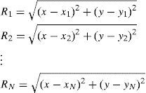
3Problem formulationLet us consider that while navigating in an environment, an OoI detects a signal from a BS with location p1 = [x1y1]T in the global map and estimates its distance R1. With this information, the position of the OoI is constrained to a circle of radius R1 and center at P1, considering that the OoI is moving on a flat surface. Similarly, receiving a signal from another BS at location p2 =[x2y2]T and its range estimate R2 will constrain its position to another circle. Concurrent reception of the two signals and the range estimation to both of the BSs will constrain the position of the OoI to two points i.e. the intersection of the two circles.
The ambiguity between the two estimates of the OoI position, given by the intersection of the two circles, can be resolved if the OoI receives signals/messages from three BSs simultaneously. Identification of a BS at p3 = [x3y3]T and its range estimation R3, will constrain the position of the OoI to a third circle. If three signals are simultaneously (assuming the OoI position is not changed) received, the OoI position is at the intersection of the three circles. Using the same argument, for an OoI receiving signals/messages from N BSs we have the following:
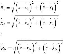
For a single circle, we can write (1) as P−PiTP−Pi=Ri2. For perfect range estimates, exact correspondence and error free locations of the BSs, the OoI position can be determined by solving (1). However, measurements are never perfect and it is very unlikely the circles will intersect at a single point. If we denote the estimated location of a BS asPˆi=xˆi yˆiT and the corresponding range estimate as Rˆi then the corresponding circle equations can be written as:
Where Pˆ=xˆi yˆiT is the estimated position of the OoI. Assuming error free BS locations and that the error in range estimation R˜;i is additive and normally distributed, we get the following Taylor’s series expansion around the estimated position:
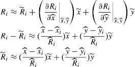
In P˜;=x˜; y˜;T represents the random error in the estimated position. Similarly, for all circles we have:
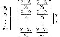
Writing in matrix form, we arrive at the following expression:
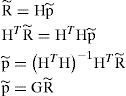
where G=(HTH)-1HT. Taking transpose of p˜; and multiplying it by itself, we have:
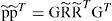
Taking expectation on both sides, we have:
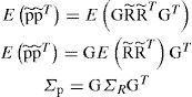
If the error in range estimation with respect to different BSs is zero mean, independent and identically distributed then ΣR=σ2IN×N⋅IN×N an N×N identity matrix. Putting this assumption in (7), we arrive at the following expression for uncertainty in the estimated position (Σp):
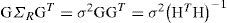
From (8) we get that uncertainty in the estimated position is proportional to (HTH)−1 and as expressed in (3) and (4), the rows of H represent the OoI to BS unit vectors. This means that for the same error in range measurement, different configurations of the OoI and BSs will result in different uncertainty for the estimated position. The matrix (HTH)−1 is called the GDoP matrix and trace ((HTH)−1) is defined as the GDoP [9][26]. One of the objectives of any positioning algorithm is to minimize GDoP. There are studies that relate GDoP to the area of polygon formed by the tips of OoI to BS unit vectors and state that minimizing the GDoP is roughly equivalent to maximizing the area of the polygon [26].
These expressions show that the uncertainty in position of the OoI is strongly dependent on locations of the BSs with respect the OoI. If the position of the OoI is changed, the overall uncertainty will also change. This means that optimal configuration of BSs for every other position of the OoI is different. It is impossible to find a configuration of BSs that will be globally optimal for all points in the application area. Therefore, the objective function needs to be formulated in such a way that error in position estimation of the OoI is minimized in an average sense. Since a minimum of three BSs are required for position estimation, it is important that every point in the area receive multiple coverage.
When the OoI receive information from N BSs, its position is the intersection of N circles given by (2). When there is error in range measurement and/or BS locations, these circles will not intersect at a single point and it is required to find a position estimate such that the overall error is minimized. When n ≤ N, where n is 2 for the two-dimensional space as assumed in our application, then the value of p that minimizes the mean square error (MSE) could be taken as the position of the OoI. Following the formulation of Zhou [27], the position estimate that minimizes the MSE can be stated as:

where SPˆ=∑i=1Np−piTp−pi=Ri2, Pˆ is the estimated position, pi is the ith reference point, N is the total number of reference points. Using the linear transformation p = q + c, the position estimate can be written as:

where, c=1N∑i=1Npi,G=−2N∑i=1NpipiT+2ccT
D=B+2ccT+ccTI,f=a+Bc+2ccTc, and I is the n × n identity matrix. Please refer to [27] for more details. We use (9) for position estimation at each point in the area. The first order statistics of this position estimation is used as a metric for selecting the appropriate configuration of the BSs for the given area.4Base station placement configurations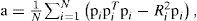

Based on our discussion in Section 2, the layout where BSs are placed on a circle may be the most effective as it avoids collinear configurations of more than two BSs and the OoI. Uniform placement of BSs on grid result in uniform coverage, whereas, placing the BSs on concentric circles tends to achieve a middle ground. We also test an arrangement that achieves uniform distribution of the BSs and at the same time avoid collinear configurations of more than three BSs within reach of the OoI. Since any area with a rectangular shape can be divided into a number of smaller squares, we propose a pattern with nested squares. The two squares have common center point and the inner square is tilted at 45 degrees with respect to the outer square. The side length of the outer square is represented by S and that of the inner square is represented by L. The vertices of the inner square are located on a distance of L/2 from the center. The nested square (NSquare) configuration is shown in Figure 1. Since the square with side length L resides inside the square with side length S, we have the following relationship: L≤S2

The NSquare can be readily extended to cover areas of different dimensions as shown in Figure 2. The value of S is dependent of the maximum range of BS. Shorter range BSs requires denser deployment of BSs and vice versa for long range BSs. Similarly, performance of the position estimation algorithm varies with the value of L for a fixed value of S. We perform extensive experimental analysis to find the optimum values based on the given criteria.

We place BSs according to the configurations stated in this section; circular (Circle), uniform (Grid), concentric circles (CCircles) and the nested squares (NSquare). Area coverage and position error are the metrics for performance comparison of different configurations. We vary the relevant parameters in each scenario and pick the best for the comparison. For example, in the NSquare we simulate the pattern for multiple value of L as discussed in the next section.
5Experimental resultsAssuming we need to localize an OoI in a rectangular area of size 600m × 300m. Using short-range BSs (coverage radius of 100m) at least twelve BSs are required to provide single coverage as shown in Figure 3. This single coverage system follows the coverage mechanism in cellular networks where the hexagon pattern is used for coverage. Now to perform localization, an OoI is required to compute its range to a minimum of three BSs simultaneously. For better positioning accuracy and protection against failure of BSs, the OoI needs range computation to four BSs. With a simple arithmetic, one can easily compute that at least 48 BSs would be required so that an OoI has access to four BSs everywhere. Now the problem is how these BSs could be placed in the area so that we have the ability to localize the OoI everywhere and the average error is minimized. Placing groups of four BSs close to each other maximizes the coverage but results in worse localization performance.

The two dimensional area where the OoI can move is represented by the two variables [x y]T. For position estimation of the OoI everywhere in the area, we take uniform samples (step size Δ) along x and y directions. The OoI is then placed at all the sampled locations and its position is estimated with respect to all BSs from whom it receives a signal. We fix the number of BSs and assume that they can be placed anywhere in the area. Our simulation maintains a record of true positions of OoI and, we implement (9) for estimating the position assuming a passive OoI. We use mean and standard deviation of the absolute error of the estimated positions for comparing the performance of different placement scenarios. Multiple trials are run and the results averaged. It is assumed that the location of BSs is error free and the range estimation error has a Gaussian distribution. We also repeat our simulations for different strength of range error to see how the performance degrades as the error grow.
As mentioned earlier that finding an analytical solution for the placement of the BSs in a way to maximize the coverage and minimize positioning error is of formidable complexity. Therefore, we evaluate representative scenarios. It is well known that a collinear configuration of the OoI and BSs result in singularity[16][18], therefore we select variation of layouts where the distribution of the BSs is more or less uniform and at the same time all the BSs and the OoI are not collinear. We place N BSs in the area. For experiments reported in this paper, we have N = 45 for the grid. For the circle, concentric circle, and nested square configurations we have N = 47.
The four different scenarios/configurations of BSs are shown in Figure 4. The number of BSs reachable from a particular point is shown as shades of grey. In the first scenario (Grid, Figure 4(a)) the BSs are placed on a uniform grid. The second (CCirlce, Figure 4(b)) and third (Circle, Figure 4(c)) configurations are circular in nature. In the second scenario, the BSs are placed on concentric circles of radius 100m and 150m. In the third scenario, the BSs are placed on circles of radius 112m. The angular displacement in the circular configurations is uniform. The nested square pattern (NSquare, Figure 4(d)) is our last scenario. In Figure 4, the signal from each BS covers a circular disk region of radius r. In our simulations, we have 10m. Since the signal from the BSs is not utilized within 10m region surrounding the BS, the location of the BSs in Figure 4 can be identified by the small circular regions. These regions have lower intensity as compared to their neighborhoods. The magic numbers in these paragraphs are derived based on repeated trials for an area of size 600m×300m. Comparison with other values is given at the end of this section.

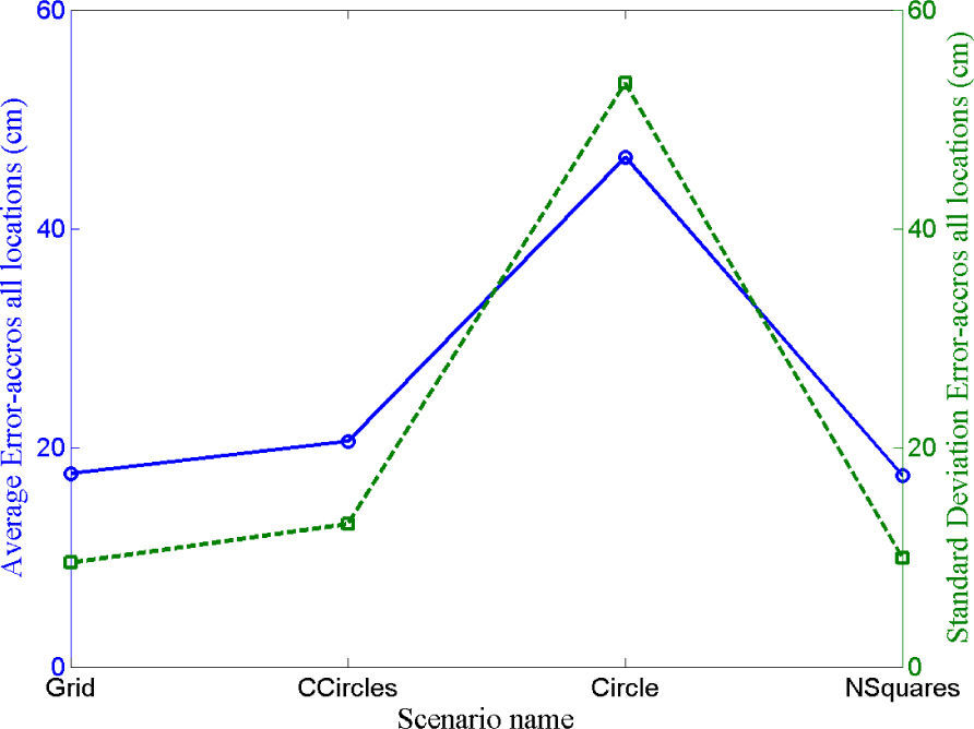
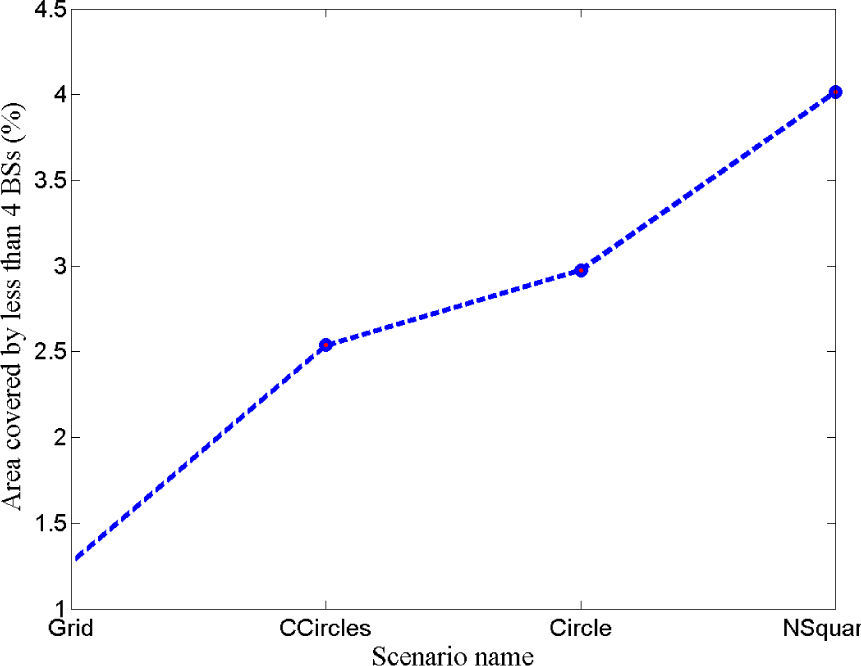
Mean and standard deviation of the absolute error in position estimation for different scenarios is shown in Figure 5. Percentage of the area that is not covered by at least four BSs is shown in Figure 6. For the results shown in Figure 5 we impose zero error on the BS locations and the range estimation error has a standard deviation of 20cm. These results clearly demonstrate that the grid and nested square configurations achieve the best performance based on the mean and standard deviation of position error. The performance of the nested square is comparable with the grid. Similarly, in terms of coverage we see better results for the grid configurations. Comparison of Figure 5 and Figure 6 leads to the conclusion that even with short range BSs the configurations that tends to place BSs uniformly results in superior performance in the average sense.


The performance of a position estimation algorithm improves when the number of BSs with respect to whom the position is estimated is increasing.
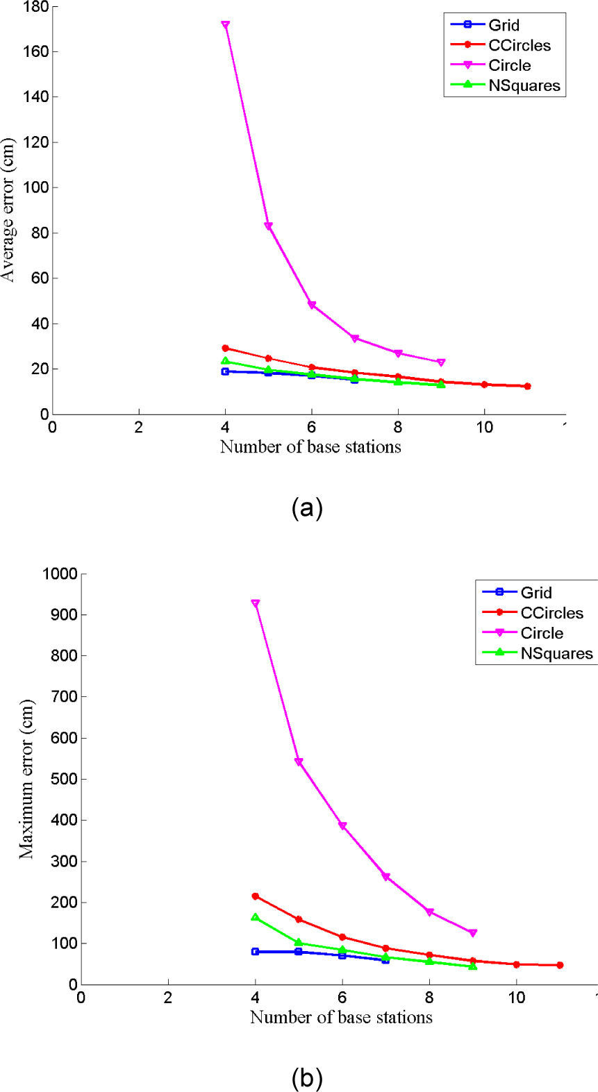
Relationship between mean error and the number of BSs used for position estimation is shown in Figure 7. It can be seen from Figure 7 that worse performance is achieved for the circle layout of the BSs and the best for the grid and nested square. For the circle layout, the error drops quickly as the number of BSs is increased. A closer look at Figure 4(c) reveals that lower numbers of BSs are available at the outer periphery and hence the error is relatively higher over there. This result is consistent with the one reported in [14] which indicates that the performance is getting worse when the OoI is outside the circle formed by the BSs. The performance of the grid and nested square layout is very close. It should be emphasized again that the grid layout is using fewer BSs as compared to the other layouts.
 average error (b) maximum error.")
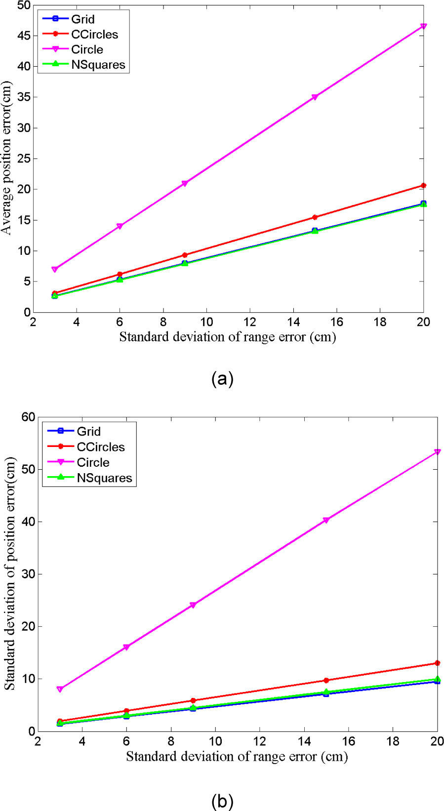
To test the sensitivity of BSs placement, we repeat the experiments by increasing the strength of range estimation error. The degradation in average performance when the range estimation error is increased is shown in Figure 8. It is clearly seen from these results that performance degradation for the scenarios that tend to distribute the BSs uniformly is lower as compared to others.
 mean (b) standard deviation.")
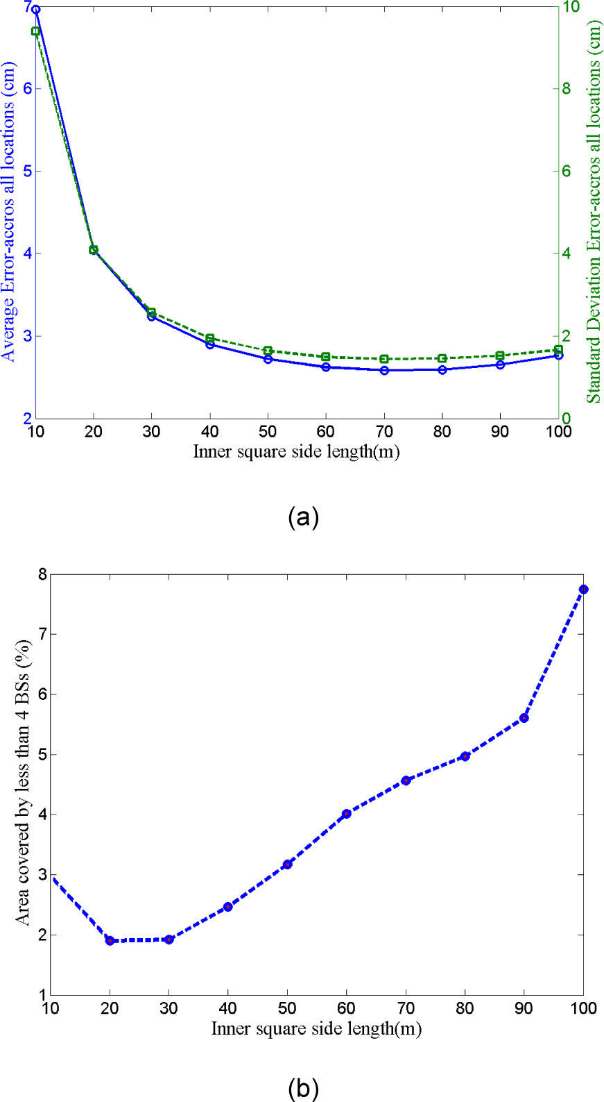
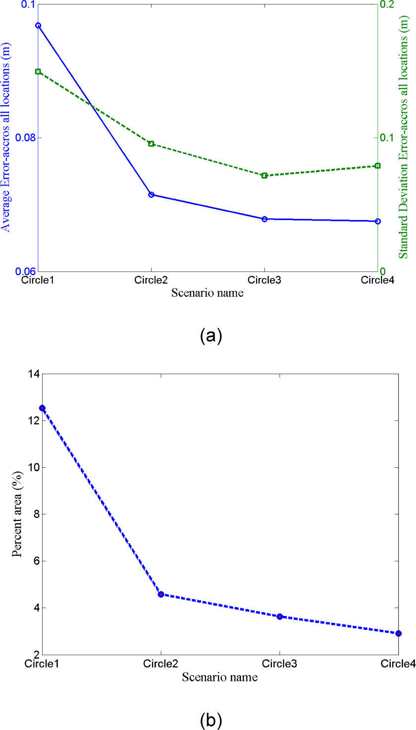
Parameter changes in each category have an effect on performance. We have performed extensive simulations by varying parameter values. Examples of the NSquare and Circle are shown in Figure 9 and Figure 10, respectively. Figure 9(a) shows mean and standard deviation of the absolute position error as a function of the size length of the inner circle. Percentage of the area not covered by at least four BSs is shown in Figure 9(b). The length of the outer square is 150m. Similarly, results for four different diameters of the circle are shown in Figure 10. In the same manner, we have tested different grid and centric circle arrangement. Layout resulting in relatively better performance in each category is then used for the final comparison shown in Figure 5 to Figure 8. In these comparison results the standard deviation of the range estimation error is 3cm.
 Overall position error as a function of side length of the inner square using Nsquare pattern (b) percentage of the area not covered by at least four base stations.")

From our simulation results, we see that for the given area consistently better performance is achieved for the grid and nested square configurations.
6ConclusionIn this paper, we investigated the placement of short range BSs for self-localization of an OoI in an area. Since the OoI can move to any point in the area, our evaluation criteria is based on the ability to localize the OoI everywhere in the area and not just at few representative locations. We choose the mean and standard deviation of the positioning error and coverage area as performance metrics. The results show that better performance in terms of mean, standard deviation of the error and coverage could be obtained by uniform placement of the BSs. The performance degradation with increasing error strength is also slower for configurations that tend to be uniform.
We intend to extend our work towards achieving better understanding of the ideal BSs placement in situations where directed antennas are being used. In such a case, we need to achieve the best coverage while employing the least possible number of BSs.
This work is supported by Auto21 (auto21.ca).