


In this paper, we propose a hybrid maximum likelihood (ML) decoding scheme for multiple-input multiple-output (MIMO) systems. After partitioning the searching tree into several stages, the proposed scheme adopts the combination of depth- and breadth-first search methods in an organized way. Taking the number of stages, the size of signal constellation, and the number of antennas as the parameter of the scheme, we provide extensive simulation results for various MIMO communication conditions. Numerical results indicate that, when the depth- and breadth-first search methods are employed appropriately, the proposed scheme exhibits substantially lower computational complexity than conventional ML decoders while maintaining the ML bit error performance.
It is well known that a significant gain in the spectral efficiency can be secured if we utilize the multiple-input multiple-output (MIMO) system when compared to the use of a single-input single-output system. The MIMO system is one of the promising techniques for next-generation communication systems because of its increased capacity without requiring consumption of excess frequency spectrum [1]. In particular, the spectral efficiency of the MIMO systems stems from the spatial multiplexing and increases as the number of antennas employed increases. Due to the increased interference among the transmit antennas or mobility of the devices [2], on the other hand, a more challenging decoding task at the receiver side is an unavoidable expense in making use of the advantages of MIMO systems comprehensively.
The problem of designing computationally efficient MIMO decoders has been addressed in many studies. Among the representative examples of computationally efficient decoders are such suboptimal decoders as the zero-forcing, nulling and cancelling, and nulling and cancelling with optimal ordering schemes [3]. With the bit error rate (BER) not equal to the ML performance, the suboptimal decoders are not appropriate in some situations to fully utilize the advantages inherent in the MIMO systems despite their low computational complexity.
Theoretically, a maximum likelihood (ML) decoder achieves the optimal BER performance for MIMO systems. The conventional full-search ML decoder inspecting all the lattice points in a tree requires a computational complexity that grows excessively fast as the number of antennas or the size of signal constellation increases. To alleviate the computational complexity of the conventional full-search ML decoder while maintaining the optimal BER performance, the sphere decoder (SD) has been proposed and analyzed in [4]. By searching over only the lattice points lying inside a hypersphere centered at the received signal point, SD reduces the search space and consequently the required computational complexity. Specifically, it is reported that, when the signal-to-noise ratio (SNR) is high and the number of antennas is small, the computational complexity of SD is comparable to that of suboptimal decoders. However, the computational complexity of SD increases significantly as the number of antennas increases or the SNR becomes low [5]. The breadth-first signal decoder (BSIDE), searching the closest lattice point based on a breadth-first search method, is proposed and shown to exhibit a lower computational complexity than SD and the optimal BER performance [6]. Nonetheless, it seems that BSIDE does not provide sufficient complexity reduction when the size of signal constellation is large. Recently, several low complexity decoding schemes were proposed employing a partial ML decoder with the successive interference cancellation detector [7] and with the chase detector [8]. However, the schemes in [7] and [8] cannot provide the optimal detection performance.
In this paper, we propose a novel ML decoding scheme, called the partition-based hybrid decoding (PHD), which first partitions the tree into several stages, and then applies depth- or breadth-first search method appropriately in each of the stages to find the ML solution. By determining a set of candidate nodes leading to the ML solution at the end of each of the stages (except for the last stage) and inspecting the more-likely candidates first, PHD can reduce the computational complexity substantially. The computational gain of PHD is shown to be more significant when the SNR is lower and when the number of antennas is larger.
The rest of this paper is organized as follows. The MIMO system model assumed in this paper is described in Section 2 and details of PHD are presented in Section 3. The computational complexity and BER performance of BSIDE, PHD, and SD are explored and compared in Section 4. Finally, Section 5 summarizes this paper.
2System modelLet us consider a MIMO system with Nt transmit and Nr receive antennas as shown in Figure 1. At the transmitter side, the input data stream is divided into Nt substreams, each of which is then transmitted through a dedicated transmit antenna over a flat Rayleigh fading channel. The channel is assumed to be constant over one transmission period but may change from one transmission to another.

Then, the baseband complex received signal r_˜;=[r˜;1,r˜;2,…,r˜;Nr]T can be formulated as

where H˜; is the Nr×Nt complex channel transfer matrix, s˜;_=[s˜;1,s˜;2,…,s˜;Nt]T is an Nt×1 complex transmitted signal vector, and n˜;_=[n˜;1,n˜;2,…,n˜;Nt]T is an complex noise vector. Here, the superscript T signifies the transpose of a matrix. The elements {h˜;i,j} of the complex channel transfer matrix H˜; are independent and identically distributed (i.i.d) complex Gaussian random variables with mean zero and variance one: we assume that all the complex channel transfer coefficients {h˜;i,j} have perfectly been estimated before the beginning of the decoding procedure at the receiver. The additive noise components {ñi} are i.i.d complex Gaussian random variables with mean zero and variance σ2 / 2 per dimension. We assume that the complex transmitted signals {s˜;i} are drawn from the constellation of an L2-quadrature amplitude modulation (QAM), where L is a power of 2.
To simplify the description of PHD, let us now convert the complex matrix and vectors in Eq. 1 into real expressions. For convenience, let M=2Nt and N=2Nr. From Eq. 1 we then have

where r_=[ℜ(r_˜;T)ℑ(r_˜;T)]T=[r1,r2,…,rN]T denotes the received signal vector,

denotes the real representation of the channel transfer matrix H˜;, s_=[ℜ{s¯_T}ℑ{s¯_T}]T=[s1,s2,…,sM]T is the transmitted signal vector in the real domain, and n_=[ℜ{n¯_T}ℑ{n¯_T}]T=[n1,n2,…,nN]T is the noise vector. Here, ℜ{·} and ℑ{·} designate the real and imaginary parts, respectively. Since s˜;i is drawn from an L2-QAM constellation, we have s_∈SLM, where it is assumed that

Performing the QR decomposition on the channel transfer matrix H when N≥M, we can rewrite Eq. 2 as [9]

where Q=[Q1Q2] is an N×N unitary matrix, R=[ri,j] is an M×M upper triangular matrix, and 0N−M,M is an all-zero matrix of size (N – M)×M. Multiplying QT=[Q1Q2]T from the left on both sides of Eq. 5, we obtain

where y_=Q1Tr_=[yi],w_=Q1Tn_, and y_′=w_′=Q2Tr_=Q2Tn_. It is noteworthy that only y_, but not y_, is dependent (or contains information) on the transmitted signal s_.
Let us now consider the ML decoding of a transmitted signal vector s_. Given a received vector r_ and the channel transfer matrix H, the distance between r_ and Hs_ is calculated as

since QQT=I, where │·│ denotes the Euclidean norm. As we have observed in Eq. 6, ‖Q2Tr_‖2=‖y_′‖2 is not dependent on s_, and therefore, the ML solution sˆ_ is obtained eventually as

If N<M, on the other hand, the channel transfer matrix is first partitioned into H=[H1, H2], where H1 and H2 are of sizes N×N and N×(M−N), respectively. Performing QR decomposition on H1, we have [9]

from Eq. 2, where Q is an N×N unitary matrix and R is an N×N upper triangular matrix. If we multiply QT from the left on both sides of Eq. 9, we obtain y_=Rs_1+QTH2s_2+n_′, where y_=QTr_, s_1=[s1,s2,…,sN]T,s_2=[sN+1,sN+2,…,sM]T, and n_′=QTn_. In order to find the ML solution sˆ_, we first fix s_2 and search over s_1 to minimize ‖y_-Rs_1-QTH2s_2‖2 and then the procedure is repeated for every choice of s_2∈SLM-N. The ML solution sˆ_ can thus be found as

In this paper, we assume that N≥M for simplicity: however, all the results in this paper can be readily extended to the situation N<M also.
3Proposed decoding scheme3.1PreliminariesUsing that the matrix R is upper triangular, the tree structure is assumed to find the ML solution sˆ_ in PHD as in other well-known decoding schemes [10]. Considering an Nr×Nt MIMO system with L2-QAM, an L-ary tree with M (=2Nt) layers starting from a root is created. The ith node in the kth layer of the tree is denoted by the vector s_k(i)=[sk,k(i),sk+1,k(i),…,sM,k(i)]T for k=1,2,…,M and i=1,2,…,LM-k+1 with s_M+1(1) denoting the root (the only node in layer M+1) of the tree. Since the elements {sj,k(i)}j=kM of s_k(i) are drawn from SL, a transmitted vector s_ can be represented by a node s_1(i) in the first layer of the tree. Figure 2 shows an example of the tree when M=4 and L=2 with S2={-12,12}.
. when ϵl=1, ϵf=0.4, N=8, and the noise is absent.")
Defining the (node) metric of a node s_k(i) as

it is clear from Eq. 8 that the goal of the tree searching in an ML decoding scheme is to find a vector in the first layer whose node metric is the smallest among {Λ(s_1(i))}i=1LM. In the context of the tree searching in this paper, other such commonly-used traditional terminology as the child node, descendant node, predecessor node, and subtree will be adopted with the usual definitions as in [11].
3.2The proposed decoding schemeThe proposed decoding scheme, PHD, first partitions the tree into several stages of layers. For a tree with M layers, we can in general partition the tree into T stages with stage i containing Mi layers, where i=1,2,…,T, T ∈ {1,2,…,M}, Mi ∈ {1,2,…,M}, and ∑i=1TMi=M. Clearly, the lth stage is composed of layers M−∑j=1I=1Mj, M−∑j=1I−1Mj−1,…,, and M-∑j=1IMj+1 in the tree. In the example of Figure 2 for instance, the first, second, and third stages are the collections {layer 4}, {layer 3 layer 2}, and {layer 1}, respectively.
In each of the stages, a depth- or breadth-first search method can be employed appropriately, and the search is restricted to the subtrees rooted from the nodes survived in the previous stage. Here, the root s_M+1(1) of the whole tree is assumed to be the only node survived prior to the first stage.
3.2.1Step 1: Determining candidates for the ML solution in the first (T-1) stagesIn each of the (T−1) stages in Step 1, a set of nodes to be used as the roots of the subtrees in the next stage is determined at the bottom layer of the stage by applying a depth-first or a breadth-first search method. The nodes survived are those with metrics smaller than or equal to the threshold DDFE2=‖y_-Rs⌣_‖2, the metric of the solution s⌣_ of the decision feedback equalizer (DFE). The merit of employing the DFE metric DDFE2 as the threshold is that the DFE requires less computational complexity than other well-known algorithms utilizing QR decomposition. By using DDFE2, it is in addition guaranteed that the ML solution is not discarded during the search in Step 1 since DML2=‖y_-Rsˆ_‖2≤‖y_-Rs⌣_‖2=DDFE2, where the ML metric DML2 signifies the metric of the ML solution sˆ_. Here, DML2 measures the metric between the ML solution in the first layer and the root of a tree, or equivalently, the square of the distance between the transformed received signal y_=Q1Tr_ and the closest lattice point among those constructed by the matrix R and signal constellation SLM.
At the end of the lth stage, a set

of Nl pairs of nodes and their node metrics at the bottom layer (that is, the layer with k=M-∑j=1IMj+1 of the stage is determined by employing appropriately a depth- or breadth-first search method for l=1,2,…,T− 1. Here, the numbers {Nl} of survived nodes are such that L∑j=1T-1Mj≥NT-1≥NT-2≥…≥N1≥1. In the (l+1)st stage, the search continues over the Nl subtrees rooted from the Nl nodes in Ωl.
When a depth-first search method is employed in a stage of Step 1, the scheme traverses toward a lower layer by adding only one child node with node metric smaller than or equal to the threshold at a time until it reaches the bottom layer of the stage or until all the child nodes of a node are explored and found to have metrics larger than or equal to the threshold. Then a backtrack occurs and the search returns to the predecessor node in the lowest layer having at least one unexplored child node, at which the depth-first search method inspects an unexplored child node with metric smaller than or equal to the threshold. The procedure continues until the depth-first search method reaches back the root of the (sub)tree with no node left unexplored.
On the other hand, when a breadth-first search method is adopted in a stage of Step 1, the scheme first computes all the node metrics in the top layer and then discards nodes with the node metrics larger than the threshold. The node metrics in the layer immediately below are then computed only for the nodes stemmed from the survived nodes. Such a procedure continues until all the nodes with node metric smaller than or equal to the threshold are found in the bottom layer of the stage.
3.2.2Step 2: Finding the node with the shortest node metric in the first layerIn the last stage, setting the threshold to DDFE2 at the beginning, the NT−1 subtrees stemmed from the NT− 1 nodes in ΩT−1 are searched by employing one of such various ML decoders based on the depth-or breadth-first search methods as the BSIDE, list sphere decoder (LSD), and SD.
As the node in the first layer with the shortest metric will be declared the ML solution, it is desired to find the node preferably without searching all the subtrees stemmed from the nodes survived in stage (T− 1). To that end, PHD will search the NT−1 subtrees in the ascending order of the node metric of the NT−1 nodes in ΩT−1 by re-arranging the nodes in ΩT−1 as

where k=M-∑j=1T-1Mj+1=MT+1. At the same time, to maximize the probability of finding the ML solution as soon as possible, PHD replaces the threshold with the metric of a node in the first layer whenever the metric is found to be smaller than the threshold.
Specifically, starting from the subtree rooted from the first node s_k[1], we search for the node with the smallest metric in the first layer. When the search over the subtree rooted from s_k[n-1] is completed, if the metric Λ(s_k[n]) of s_k[n] is compared to be larger than the threshold (which might have been changed from the starting value DDFE2 in the meantime), the node of which the metric became the threshold is declared the ML solution and the search is terminated. This is based on the fact that all the descendant nodes of {s_k[j]}j=nNT-1 will have node metrics larger than the shortest node metric found by that moment. The procedure of inspecting more-likely subtree (stemmed from a node with smaller metric) first and appropriately updating the threshold maximizes the probability of finding the ML solution as soon as possible, and consequently, reduces the computational complexity by preventing us from unnecessarily searching hopeless subtrees.
In contrast to conventional decoding schemes, in which only one search method is employed for the search over the entire tree, PHD enables us to employ various search methods adaptively in each of the stages of the partitioned tree when such parameters in the decoding environment as the SNR, number of antennas, and size of signal constellation change. By employing appropriate search methods in the right stages, PHD can maximally exploit the advantages of several search methods and accordingly reduce the computational complexity. In addition, as a natural advantage of the tree partitioning, PHD searches more-likely candidate subtrees first and terminates the searching process as soon as the ML solution is found, resulting in further reduction of the computational complexity.
4Performance evaluation4.1Analysis of computational complexityThe number of multiplications (NOMs) is a useful index accepted widely in illustrating the computational complexity of a decoding scheme [12], In this paper also, the computational complexity of PHD is investigated and compared with those of other ML decoding schemes in terms of the number of multiplications.
At the beginning of PHD, the QR decomposition of H is performed and y_=Q1Tr_,s⌣_, and DDFE2=‖y_-Rs_‖2 are computed. The number of multiplications required for the QR decomposition is approximately NM2– M3/ 3 [13]. Computing y_,DDFE2, and s⌣_ require NM multiplications, M(M+3) / 2 multiplications, and M divisions, respectively [6]. Assuming that a division requires the same amount of computational complexity as a multiplication, the total number of multiplications required for these computations is thus

Note that Eq. 14 is the number of multiplications required independent of the SNR and size of signal constellation.
The computational complexity of PHD can be decided by adding the number Eq. 14 to the total number of multiplications in the T stages. The number of multiplications in a stage will of course depend on the decoding scheme employed and the number of nodes with metric smaller than or equal to the threshold in the stage. Now, the number of nodes with metric smaller than or equal to the threshold is a random variable since it is a function of the channel transfer matrix H and received vector r_, both of which are clearly random variables depending on the SNR. Taking in addition into account that the exact path of a decoding scheme over the tree is unpredictable, it is obvious that the number of multiplications (of any decoder) will differ from transmission to transmission. Consequently, it is impossible to acquire an exact closed-form expression for the number of multiplications of a decoding scheme in general. In this paper, therefore, the number of multiplications of various decoding schemes are obtained and compared by means of averaging over a large number of repetitions via computer simulations.
4.2Simulation results and discussionsWe now evaluate and compare the computational complexities of BSIDE, PHD, and SD in terms of the average number of multiplications over 106 iterations via computer simulations. For simulations, we consider Rayleigh fading channels with additive white Gaussian noise [14], [15]. The BER performance characteristics of BSIDE, PHD, and SD will also be shown when appropriate to confirm that they all have the ML performance. Additional interesting characteristics of PHD will be discussed in terms of the relationship between the configurations of stages and NOMs in several MIMO transmission scenarios.
In all the simulations herein, the SNR is defined as E{‖Hs_‖2}/E{‖n‖2}, where E{·} denotes the expectation. In specifying the structure (configuration) of PHD, we will use the notation PHD [{Aj(Mj)}j=1T] to denote that search method Aj is employed in the jth stage composed of Mj layers for j=1,2,…,T. In representing search methods {Aj}, the symbols ‘BF’, ‘BS’, ‘LS’, and ‘SD’ will stand for the breadth-first search, BSIDE, LSD, and SD, respectively. It is noteworthy that among these four search methods, ‘BS’ and ‘SD’ can be used only in Step 2 of PHD, ‘BF’ can be used only in Step 1 of PHD, and ‘LS’ can be used both in Steps 1 and 2. Consequently, there may exist six possible combinations of search methods in Steps 1 and 2 of PHD. In the simulations, we set the initial searching radius of LSD and SD to DDFE and assume the computational complexity of a square root is the same as that of a multiplication.
4.2.1On the numbers of stagesFigure 3 shows the average number of multiplications of PHD as a function of the number T of stages when various search methods are adopted in PHD and Nt=Nr=4. It is interesting to observe, when the search methods are all the same in the first (T−1) stages, that (1) the computational complexity of PHD depends mainly on the search method and the number of layers in the last stage and (2) the changes in the number of stages and layers in the first (T−1) stages barely influence the computational complexity. For example, the computational complexities of PHD[LS(6),SD(2)] and PHD[LS(2),LS(3),SD(3)] are almost the same as that of PHD[LS(2),LS(2),LS(2),SD(2)] and PHD[LS(2),LS(1),LS(1),LS(1),SD(3)], respectively. Although we have shown the results for only a limited number of combinations for the search methods, we have confirmed that other combinations also result in the same tendency.
 LS and SD, (b) LS and BS, (c) BF and LS, and (d) BF and BS when L=4 and Nt=Nr=4.")
From this observation, we can infer that, in designing or choosing the configuration of PHD, a number of contiguous stages with the same search method in Step 1 may be merged into one stage with the common search method without affecting the overall computational complexity. In other words, unless two or more search methods are employed in Step 1, partitioning a tree into two stages should be a reasonable choice.
4.2.2On the numbers of layers in stagesIn Figure 4, for all possible (=six) combinations of search methods in the two stages, we have shown the dependence of the computational complexity of PHD on the numbers M1 and M2=8 – M1 of layers in the two stages when Nt=Nr=4, L=4, and T=2. Clearly, the computational complexity of PHD depends on the specific configuration and varies as the search methods and numbers of layers in the two stages change: yet, the difference in the numbers of multiplications among the various configurations of PHD decreases rapidly as the SNR increases. Similar observations have been made for other values of L also, which are not included in this paper for a space reason.

Although different choices of the numbers of layers in the two stages will result in different level of computational complexity, M1=M2=M / 2 is not an unreasonable choice in the investigation of the computational complexity of PHD in terms of the average number of multiplications. Intuitively, a larger M1 would result in more nodes survived in the first stage, more trees to search in the second stage, and consequently, higher complexity; similarly, a larger M2 would incur ‘longer’ trees in the second stage and consequently higher complexity. From now on, taking this observation into account, let us focus on PHD which partitions the tree into two stages with equal number of layers. It should be mentioned, however, that values of M1 other than M / 2 might be more beneficial depending on specific applications.
4.2.3Complexity comparisons of various decoding schemesFigure 5(a) shows the BER performance of BSIDE, LSD, PHD, and SD with two transmit and two receive antennas when the modulation order L varies. It is clearly confirmed that BSIDE, LSD, PHD, and SD all possess the ML BER performance. The average numbers of multiplications of BSIDE, LSD, PHD, and SD in three modulation schemes (4-, 16-, and 64-QAM) are shown in Figures 5(b)-(d). In these figures, it is clearly observed that PHD generally outperforms LSD and SD in most cases, and also outperforms BSIDE when the value of L is large. Furthermore, it is observed that the gain in the computational complexity of PHD over those of other schemes is generally more substantial when the SNR is low and the number of antennas is large. Similar observations can be made in Figure 6, obtained when the numbers of the transmit and receive antennas are four.
![BER performances and average NOMs of BSIDE, LSD, PHD [A1(2),A2(2)], and SD: BER performances (a) when L=2,4,8 and Nt=Nr=2 and average number of multiplications (b) when L=2 and Nt=Nr=2, (c) when L=4 and Nt=Nr=2, and (d) when L=8 and Nt=Nr=2.](https://static.elsevier.es/multimedia/16656423/0000001100000002/v2_201505081627/S1665642313715311/v2_201505081627/en/main.assets/gr5.jpeg?xkr=ue/ImdikoIMrsJoerZ+w997EogCnBdOOD93cPFbanNcX6PcOHo8VDqRKrp6xHZ/NlPxKUvo805ICrHlplwxcm7hYIESfjCCTNDlVokL+8rPPuufSpcyEsd/mUwG8Iwv+zUCyXv4fls7nDq1SHxKwx7eOGqQzRiFE7jdQTo7vIMciL3PAQeTsl7ljJNcVV1/k1NxEl43SI2N4C0s/AYZ17MTlCNheEh1oAA58daahWv5+rDlvZco9kiRLRpJBBgGuIJYq9fLYVDcp7I9Y28p9geqr51lF9F+y+nYqR4MRcbCFdVGJEJzXfqz0zPjr7E7qE0XaNCwIlCB0ISgxtPCJ+Q== "BER performances and average NOMs of BSIDE, LSD, PHD [A1(2),A2(2)], and SD: BER performances (a) when L=2,4,8 and Nt=Nr=2 and average number of multiplications (b) when L=2 and Nt=Nr=2, (c) when L=4 and Nt=Nr=2, and (d) when L=8 and Nt=Nr=2.")
![BER performances and average NOMs of BSIDE, LSD, PHD [A1(4),A2(4)], and SD: BER performances (a) when L=2,4,8 and Nt=Nr=4 and average number of multiplications (b) when L=2 and Nt=Nr=4, (c) when L=4 and Nt=Nr=4, and (d) when L=8 and Nt=Nr=4.](https://static.elsevier.es/multimedia/16656423/0000001100000002/v2_201505081627/S1665642313715311/v2_201505081627/en/main.assets/gr6.jpeg?xkr=ue/ImdikoIMrsJoerZ+w997EogCnBdOOD93cPFbanNcX6PcOHo8VDqRKrp6xHZ/NlPxKUvo805ICrHlplwxcm7hYIESfjCCTNDlVokL+8rPPuufSpcyEsd/mUwG8Iwv+zUCyXv4fls7nDq1SHxKwx7eOGqQzRiFE7jdQTo7vIMciL3PAQeTsl7ljJNcVV1/k1NxEl43SI2N4C0s/AYZ17MTlCNheEh1oAA58daahWv5+rDlvZco9kiRLRpJBBgGuIJYq9fLYVDcp7I9Y28p9geqr51lF9F+y+nYqR4MRcbCFdVGJEJzXfqz0zPjr7E7qE0XaNCwIlCB0ISgxtPCJ+Q== "BER performances and average NOMs of BSIDE, LSD, PHD [A1(4),A2(4)], and SD: BER performances (a) when L=2,4,8 and Nt=Nr=4 and average number of multiplications (b) when L=2 and Nt=Nr=4, (c) when L=4 and Nt=Nr=4, and (d) when L=8 and Nt=Nr=4.")
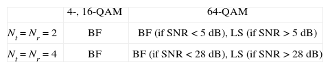
Based on the observations from the simulation results in the figures considered so far, we can make the following observations. (1) For a fixed search method in the second stage, ‘BF’ in the first stage produces lower computational complexity than ‘LS’ when Nt=Nr=2,4 and L=2,4: when L=8, we can make the same observations at lower SNR, but ‘LS’ becomes the preferred choice as the SNR gets higher. (2) For a fixed search method in the first stage, ‘BS’ in the second stage would be the first choice when L=2, and ‘LS’ would become our preference for the search method in the second stage as L gets larger. Such a dependence of the computational complexity of PHD on search methods is a natural consequence of the intrinsic of the depth- and breadth-first algorithms. We have summarized these observations in a somewhat quantitative manner in Tables 1 and 2.
In passing, we would also like to mention that, if a common search method is employed in the second stage, the numbers of multiplications from various configurations of PHD are almost identical irrespective of the search methods in the first stage when the number of antennas and/or the size of signal constellation are large.
5Concluding remarkFor applications in MIMO systems, we have proposed a novel ML decoding scheme called PHD, which provides significant gain in the computational complexity compared with conventional ML decoding schemes. The proposed decoding scheme partitions the tree into several stages, in each of which a depth- and breadth-first search method is employed appropriately. The partitioning of a tree proposed in this paper plays a key role in the proposed decoding scheme, allowing us to appropriately and fully make use of the advantages of several search methods. The proposed decoding scheme has flexibility in choosing the number of stages, the number of layers in each of the stages, and the search method in each of the stages.
From simulation results, it is confirmed that the proposed decoding scheme with proper configurations has considerably lower computational complexity than conventional ML decoders while maintaining the optimal BER performance. In addition, it is observed that the computational complexity gain of the proposed decoding scheme increases as the SNR gets low and the number of antennas increases.
AcknowledgementsThis research was supported by the National Research Foundation (NRF) of Korea under Grants 2012-0005066 and 2012R1A2A2A01045887 with funding from the Ministry of Education, Science and Technology (MEST), Korea, by the Information Technology Research Center (ITRC) program of the National IT Industry Promotion Agency under Grants NIPA-2012-H0301-12-1005 and NIPA-2012-H0301-12-2005 with funding from the Ministry of Knowledge Economy (MKE), Korea, and by National GNSS Research Center program of Defense Acquisition Program Administration and Agency for Defense Development.