Crude oil, “the blood of industry” plays an irreplaceable role in the field of industrial production. The fluctuation in oil prices directly affects metal mining and processing, which in turn affects the dynamic development of the nonferrous metal market. This study examines the dynamic connection between international crude oil and China's nonferrous metal market using a change-point detection copula method. Under hypothesis testing, the change points in the dynamic connection are well detected using our method. The results show that the occurrence of change points may be related to the production policy of the Organization of Petroleum Exporting Countries (OPEC). Information about the connection before the change points will obscure the useful information, resulting in inaccurate knowledge about the dynamic connection. In addition, the connection has a profound impact on return forecasts. The test results based on sample data from the post-change point are more likely to accept the null hypothesis. This accuracy of the return forecasts based on sample data from the post-change point is attributed to the exact establishment of the dynamic connection between crude oil and nonferrous metal market. When returns are forecast accurately, useful market information can be developed into “good knowledge” about the dynamic connection. Hence, the connection before the change points makes little contribution to forecast returns; the useful information for forecasting is the connection starting from the change points. This “good knowledge” about the dynamic connection is conducive to accurately predicting returns, thereby solving the relation between risk prevention and sustained development.
International oil prices have rebounded continuously and rose by nearly 30% by 2020. Several large fluctuations in international oil prices are connected to corresponding historically major financial crises or regional conflicts. Crude oil is the main energy source for industrial activities in world economies, and its price fluctuations are bound to have a profound impact on the development of the global economy. The development of the Belt and Road Initiative maintains a link between China and other countries along the routes, and nonferrous metals have been widely used in China's industrial production and infrastructure construction. As metals with the strongest financial attributes, nonferrous metals in China are inextricably associated with the exploitation of crude oil. First, in terms of raw materials, oil prices directly affect the mining, processing, and refining of nonferrous metals. Second, with world economic globalization, the dramatic change in crude oil prices will undoubtedly impact the output and prices of nonferrous metals. Finally, nonferrous metals, as substitutes for oil, will become targets for investors when oil prices continue to rise. Therefore, an in-depth study of the dynamic connection between the international crude oil market and China's nonferrous metal market is particularly important for measuring financial risks, improving the establishment of risk management policies, and rationally planning asset allocation.
Early literature on international crude oil and metal prices supports the idea that the changing trend between them is equidirectional (Baffes, 2007; Lescaroux, 2009; Zhang & Wei, 2010). From this perspective, the correlation between oil and metal prices remained high because of common shocks to inventory levels. This behavior weakens once the influences of supply and demand are filtered out. However, owing to differences in data and research methods during different periods, the relevant conclusions were not exactly the same. Recent studies have not only confirmed the significant spillover effect of oil price shocks on the gold and silver markets (Reboredo & Ugolini, 2016), but have also provided empirical evidence on the asymmetric impact of their positive and negative shocks on metals market volatility (Dutta, 2018). These conclusions on the relationship between crude oil prices and metal prices have produced considerable changes.
Ultimately, we should be concerned with the following research questions based on the above discussion. First, does a dynamic connection exist between crude oil and the nonferrous metal market? Second, if it exists, does this dynamic connection play an important role in forecasting returns?
In this study, two research objectives were formulated to answer these two proposed questions. First, we construct a nonlinear dynamic connection to explain the relationship between international crude oil and China's nonferrous metal market. Second, we examine the role of the dynamic connection in forecasting the returns of the two markets. Thus, we explore the “good knowledge” about the dynamic connection that favors forecast accuracy.
Our contributions are twofold. First, we develop a change-point detection copula method to explain the dynamic connection between international crude oil and China's nonferrous metal market, which can reveal the structural break characteristics of the connection. We suppose that the connection before the change points will obscure the useful information if there are change points. “Good knowledge” about the dynamic connection is formed as the real connection stems from the information from the nearest change point, rather than all the information in the process. Second, we explore the good knowledge about the dynamic connection to forecast returns. It prevents useful information in the dynamic connection from being fully covered. It is difficult to conclude that full information is consistently better than useful information in promoting good knowledge formation.
The remainder of this paper is organized as follows. The following section covers the related literature and the theoretical framework. The “Methodology” section presents the methodology used in the analysis. The “Data and descriptive statistical analysis” section describes the data and its descriptive statistical analysis. The “Empirical results” discuss the empirical results and their interpretations. Finally, the last section draws conclusions and outlines directions for further research.
Literature reviewDynamic connectionThere is an expansive literature describing the connection between financial markets that is the concern here Sklar (1959). first used the word “Copula” to denote a function, which “connects” univariate distribution functions to form multivariate distribution functions. The copula can accurately describe the connection between variables, so it is used to examine the connection between two markets. This method was further applied to investigate the static and dynamic connections between various markets (Yao & Sun, 2018; Albulescu et al., 2018). Previous studies specify that static copula is a significant method in the Eurozone and non-Eurozone stock markets (Boubaker & Sghaier, 2013; Bartram & Wang, 2015; Mensah & Premaratne, 2018). The characteristics of connections between stock markets have generally been examined from the time-invariant perspective of overall economics rather than from the perspective of stock market uncertainty Uddin et al. (2020). used a time-varying copula approach to examine the characteristics of risk spillovers between the US stock market and precious metals (gold, silver, and platinum) and oil. Accounting for time horizon factors, Mensi et al. (2021) analyzed the connection between the energy prices (natural gas, gasoline, and WTI crude oil) and major oil exporting and importing MENA stock markets. These studies limited the application of the copula method in bivariate cases; binary copula was no longer suitable for describing connections in multivariate cases.
The role of vines in mathematical graph theory can be used to explain the fundamentals of associations (Philipson, 2020) Bedford and Cooke (2001). proposed a vine structure model for random variables, which allowed high-dimensional joint distributions to be decomposed into a set of bivariate copulas using copula specifications with different connection features Bekiros et al. (2015). modeled the connection between the investment portfolio by vine copula during three periods (i.e., pre-, mid-, and post-financial crisis), and used five risk metrics to optimize investment portfolio risk Yu et al. (2020). combined a vine copula model with an analysis of structural breaks to examine the dynamic connection between oil and stock markets; the vine copula flexibly captures connections in multivariate cases. Nevertheless, various factors in the crude oil and nonferrous metal markets are changing rapidly. With major political and economic issues, it was inappropriate to use single-structure and single-parameter copula models to describe the dynamic connections between different markets (Cuaresma et al., 2019).
A financial market is subjected to the external impact of macro-control policies, which bring financial risk with structural change characteristics. It is essential to determine the structural change points using objective statistical indicators Dias (2004). discussed structural change points using the maximum likelihood approach for specific copula families. This method can be employed to determine the existence of structural changes in the connection, and a significant number of empirical studies have shown that change points indeed exist in the connection between financial markets (Ye et al., 2012; Block et al., 2015; Manner et al., 2019) Franco and Esteves (2020). also emphasized that many aspects of the dynamics of connections require further study.
These authors emphasized the role of detecting the change point in a dynamic connection. The detection of change points could reduce the selection error of change points caused by subjective judgment to more accurately describe the dynamic connection between the asset portfolio in different time periods. Therefore, there is an urgent need to develop good knowledge about dynamic connections from useful information using a new method.
The role of dynamic connection in forecasting returnsThe role of static connections in forecasting returns is usually reflected in two aspects: risk measurement and portfolio optimization. With respect to risk measurement, some authors have investigated the impact of connections on forecasting returns, concluding that the accuracy of VaR always benefits from correct connections among different markets (Zhang et al, 2014; Shahzad et al, 2016; Segnon & Trede, 2018; Kumar et al., 2019). With respect to portfolio optimization, several studies have examined the efficient portfolio, considering that the portfolio weights are subject to a static connection (Low et al., 2013; Karmakar & Paul, 2019).
Ruoslahti (2020) emphasized that interdependence is one of the most important elements in innovation projects. While the above literature emphasized the influence of static connection on forecasting returns, this work was extended by Ji et al. (2019) when analyzing the issue of the possible dynamics in the connection. They analyzed the dynamic dependence between WTI crude oil and the exchange rates of the United States and China, providing evidence of a significant asymmetric spillover effect Chen and Qu (2019). investigated the leverage effect and dynamic correlation between international crude oil and China's precious metals (gold, silver, and platinum) and used the BP test to explore the impact of macroeconomic shocks on international crude oil and precious metals in China Manner et al. (2019). proposed a method for detecting structural change points in the factor copula model, and studied the structural change points in the dependent relationships among 32 industries. Their results suggest that the detection of change points in dynamic connections is important for return forecasts Li and Li (2021). explored the dynamic connection between WTI oil and the Chinese energy stock index (300ENI) using a binary segmentation procedure to detect the change points of copula families.
Current literature has found a dynamic connection between international crude oil and metal prices. These studies only focused on the analysis of this feature and did not form it into useful knowledge for predicting returns. Given that dynamic connections play a significant role in forecasting returns, change points may govern the connections between financial markets. The detection of change points in dynamic connections is a key factor that motivates useful information for forecasting returns. Therefore, a new method is developed in this study to form good knowledge about dynamic connections, which further improves the accuracy of return forecasts.
MethodologyTo study the connections between the international crude oil market and the six nonferrous metal markets in China requires exploring the respective characteristics of individual markets and whether a dynamic connection exists between them. This section introduces three aspects. First, we introduce a method for describing the marginal distribution. Second, we develop a change-point detection copula method to explain the dynamic connection between international crude oil and China's nonferrous metal market, thus forming good knowledge about the dynamic connection. Finally, returns are forecast based on previous knowledge, and the accuracy of the returns depends on the VaR test.
Marginal distributionThe description of proper marginal distribution characteristics is an important basis for describing dynamic connections. Most studies show that GARCH-type models can capture the common characteristics of financial data, such as volatility clustering. However, it is difficult to measure the leverage effect of financial assets using a GARCH model Lee and Lin (2011). show that the GJR-GARCH model can fully describe the characteristics of autoregression, heteroscedasticity, and the leverage effect of returns. Therefore, the AR(1)-GJR-GARCH(1,1)-skewed-t model was used to fit the marginal distribution of daily returns. The model is:
where rt and rt−1 are the returns in the t-th day and (t-1)-th day, respectively. η0 is the mean of the autoregressive terms of returns. η1,α,β is constant, and α,β is greater than 0. γ is the leverage coefficient used to express the asymmetry of volatility. σt2 is the conditional variance. I(εt−1<0) is an indicator function. When εt−1<0 is used, it takes 1; otherwise, it takes 0. zt is a standardized residual term. This study assumes that the residuals follow skewed-t distributions. Thus, we can determine the respective characteristics of the individual markets.Change-point detection method based on copula functionThe distribution characteristics of one market are the groundwork for studying the dynamic relationship between markets. This section describes the development of a change-point detection method based on the copula function. Assuming that the sample size is n, the observation data for variables X and Y are (x1,y1),···,(xn,yn). C(u,v;Θ) is a function of the variables X and Y, and Θ is the set of all parameters of the copula function. In addition, assuming that there is only a change point, the null hypothesis and alternative hypothesis can be expressed as:
where θi∈Θ,i=1,2,⋯,n. In this study, the copula function contains only one parameter. If the null hypothesis is rejected, k*is the time of change in the dependence.If there is only one variable structure point and k*=kis known, then the following log-likelihood ratio statistics can be written according to the copula maximum likelihood function:
where Λ(k)=supθ∈ΘΠ1≤i≤nc(F(xi),G(yi);θ)sup(θθ)∈Θ×ΘΠ1≤i≤kc(F(xi),G(yi);θ)ΠkWhen the value of the statistic Zn is large enough, the null hypothesis can be rejected. That means there is a structural change point in LRk, and the change point time is the location of the maximum value taken.
If k* is unknown and the statistic Zn is large, the null hypothesis can be rejected. This means the model has a change point. According to the inference of Csorgo and Horvath (1997), the asymptotic distribution of Zn1/2 is
where n is the number of observations, and Γ(·) is the gamma function. mis the number of parameters that can change under this assumption. The copula functions in this study all contain only one parameter, namely, m=1. When h(n)=l(n)=(logn)3/2n is obtained through Monte Carlo simulation, Eq. (8) exhibits the fastest convergence speed. The estimation of the change-point time k* is:If one sequence has multiple change points, it can be detected using the bisection method proposed by Vostrikova (1981). The specific steps are as follows. First, we detect a single change point for the full sample. If there is no change point, then the null hypothesis is accepted. If there is a change point, the change point divides the full data into two subsamples. For each subsample, we detect the second change point according to the first step and continue this process until there is no change point in each subsample.
If the null hypothesis in Eq. (4) is rejected, the alternative hypothesis in Eq. (4) is accepted. Θ in the copula function C(u,v;Θ) of variables X and Y is time-varying. k* is the time of change in dependence. The connection between X and Y based on the full-sample data fails to reflect a dynamic nature. The connection before the change points will cover useful information, resulting in inaccurate knowledge about the dynamic connection. The real connection is the information from the nearest change point rather than all the information in the whole process. This “good knowledge” about the dynamic connection is formed here to forecast returns. Hence, the connection before the change points makes little contribution to forecast returns, whereas the useful information for forecasting is the connection starting from the change points.
Return forecasts and testingWe forecast returns based on previous good knowledge and the accuracy of the returns depends on the VaR test. First, we introduce the main steps in the return forecasts. Second, we present the basic concepts of VaR and the backtesting method.
Return forecasts. To investigate the impact of connections on forecasting returns, this section uses sample data from the post-change point. Specifically, we calculate the returns on the crude oil and nonferrous metal markets combined with the rolling simulation estimation method. The main steps based on copula change point detection knowledge are as follows.
Step 1: The Monte Carlo simulation method is used to simulate random numbers according to the estimated parameters of the copula, which is obtained by good knowledge about the dynamic connection.
Step 2: The simulated value of the standardized residuals can be obtained by an inverse probability integral transformation of random numbers.
Step 3: The simulated values of the residuals are substituted into the GARCH model to obtain the simulated value for each return.
Step 4: The weights of the asset portfolio are selected to obtain portfolio returns.
It is noteworthy that the parameters in the change-point detection method are estimated using sample data from the post-change point rather than the full sample in Step 1. In other words, returns are forecast using information from the nearest change point.
The backtesting method. VaR refers to the maximum possible loss of financial asset or asset portfolio value in a specific period in the future under a certain confidence level. It describes the quantile of the expected distribution of returns. In addition, it is a market risk metric. It can be mathematically defined as:
where rt is financial asset returns at time t. 1−β is the confidence level and VaRβ,t is the value at risk of financial assets at the given confidence level. If the distribution function Ft(·)of the return rt is continuous, then VaRβ,t=Ft−1(β). VaR is mainly affected by the assumptions of duration, confidence level, and distribution of financial returns.The VaR of the financial asset portfolio can be expressed as:
Eq. (11) assumes that the financial asset portfolio contains n assets, and rit is the return of the i-th asset in the portfolio at time t. wi is the weight of the i-th asset in the portfolio, and the sum of the weights of each asset ∑i=1nwiis equal to 1.
The VaR value is essentially the quantile corresponding to a certain probability of the distribution function of the assets or portfolio returns. It quantifies the risks of different financial assets, institutions, and markets into a simple value.
To test the accuracy of VaRs based on different models, it is necessary to backtest on VaRs Kupiec (1995). proposed a likelihood ratio (LR) test based on the VaR failure rate, that is, the unconditional coverage test. It is used to test whether the failure rate is equal to a given significance level or to test whether there is a significant difference between the actual number of failures and the expected ones. The principle of the unconditional coverage test is as follows.
Assuming that there areTobservations in the sample, we compare the VaRs of financial institutions with the corresponding actual returns. A situation in which the actual return is less than the predicted VaR is called a VaR violation event. The "hit sequence" of the VaR violation events of financial institutions at the significance level β can be defined as:
where Hitt(t=1,···,T) equals one when a violation occurs. Otherwise, it is equal to 0. If a model that is used to calculate VaR under the significance level of β is sufficiently accurate, the "hit sequence" will follow the Bernoulli distribution with parameter β. Thus, the following null hypotheses are proposed:This hypothesis is equivalent to testing whether the probability π of Hiti=1 is significantly different from β. The hypotheses can be written as follows:
Under the null hypothesis, the likelihood function L(β) is:
where T is the total length of the "hit sequence". T1 is the number of violation events and T0is the number of complementary events. The estimated value of π is π^=T1T. If the null hypothesis of Eq. (13) or (14) is correct, the unconditional coverage test statistic LRUC is:If LRUC exceeds the critical value of the χ2(1) distribution, the null hypothesis is rejected and the VaR value is considered inaccurate. Otherwise, the null hypothesis is accepted and the VaR value is considered accurate, which means that this model can accurately calculate VaR. Furthermore, the accuracy of returns depends on the VaR test. The accuracy of the returns is verified when the null hypothesis is accepted. It is considered that a good knowledge of dynamic connections is reasonable.
Data and descriptive statisticsIn the empirical analysis, the GJR-GARCH-skewed-t model is constructed to fit the marginal distributions of international crude oil (Brent crude oil) and six nonferrous metals (copper, aluminum, lead, zinc, tin, and nickel). The binary copula functions between international crude oil and each nonferrous metal market are estimated, and the change points of the connection between crude oil and nonferrous metal market are tested using the change-point detection copula method. Thus, the full sample is divided into two parts. We also use the Monte Carlo and rolling simulation methods to calculate the VaRs to measure the risk of the two markets in terms of the sample data from the post-change point. Finally, the results of backtesting are compared with those of the VaRs in terms of the full sample.
This study uses the Brent crude oil futures prices to represent the international oil prices and selects the six specific nonferrous metal market prices indices (SMMI) of copper, aluminum, lead, zinc, tin, and nickel published by the Shanghai Nonferrous Metals Network during the same period. There are seven variables. To measure the connection between the international crude oil and the Chinese nonferrous metal market requires first conducting a descriptive statistical analysis of each variable's returns. The sample period is from March 27, 2015, to April 6, 2021. After excluding missing and unmatched data, it covers a total of 1467 observations. The data are obtained from the Choice Financial Terminal.
This study uses the log return of each variable, and it is defined as:
where rt is the log return of variable. pt and pt−1 are the daily closing prices of the variables at t and t−1, respectively. Finally, we get 1466 groups of sample returns. The results of the descriptive statistical analysis of the daily log returns are presented in Table 1.Descriptive statistical results for the daily returns of each variable.
Note: (1) JB test *** means rejecting the null hypothesis of Normal distribution at a 1% significance level; (2) ADF test *** means rejecting the null hypothesis of unit roots at 1% significance level; (3) The values in the brackets correspond to the p value of the test statistic.
As shown in Table 1, the highest average daily return for each variable is 0.24. The average daily returns of tin and nickel are greater than 0.1, while the average daily returns of the other variables are below 0.1. The standard deviation describes the degree of data dispersion. The larger the standard deviation, the greater the data fluctuation. Compared with other nonferrous metals, the standard deviation of nickel is 82.80, indicating that nickel fluctuates more than other industries during the sample period. The skewness and kurtosis reflect the symmetry and concentration of data, respectively. The returns of the international crude oil, copper, and tin industries are negatively skewed, suggesting that these three industries have more negative returns. The four nonferrous metal returns, aluminum, lead, zinc, and nickel, are skewed. The degrees are all positive, which means that it is easier to observe positive returns for these four nonferrous metals. The kurtosis of each return is greater than three, which is in line with the typical leptokurtosis and fat-tail characteristics of financial time series. The JB test statistics show that the daily returns of each variable reject the null hypothesis of "Returns follow the normal distributions" at a significance level of 1%. Thus, normal distributions cannot capture the performance of returns. The ADF test results show that the statistics are less than the critical values at the 1% significance level, indicating that each series has no unit roots, that is, all returns are stationary series. Additionally, the ARCH test statistics show that they are significant at the 99% confidence level. In other words, volatility clustering affects each variable's daily returns. Therefore, it is necessary to establish a marginal distribution model of GARCH for each return with the characteristics of leptokurtosis, fat-tail, and asymmetry.
Empirical resultsIn this section, we first estimate the parameters of the marginal model for each industry and present the optimal copulas between the international crude oil market and China's nonferrous metal market. We then detect the change point of the connection between the two markets and accurately predict the VaR of the two markets based on sample data from the post-change point. Finally, we compare the performance of these two methods using the p values of the backtesting VaRs.
Marginal model resultsBefore analyzing the nonlinear connection between the international crude oil and nonferrous metal market, it is necessary to first fit the marginal distribution of each variable. According to the descriptive statistical results, the daily returns of the two markets have the characteristics of leptokurtosis and fat-tail, autocorrelation, heteroscedasticity and volatility clustering. In this study, AR(1)-GJR- GARCH(1,1) is selected to fit the marginal distribution of the sample data, and the skewed-t distribution is selected for the distribution of the residuals. Table 2 presents the marginal model estimates.
The parameter estimates of AR(1)-GJR-GARCH(1,1)-skewed-t model.
Note: ***, **, and * indicate significant at the level of 1%, 5%, and 10%, respectively.
Table 2 presents the fitting results of the GJR-GARCH(1,1)-skewed-t model for each variable. The results show that each parameter is significant and that the returns of each industry exhibit volatility clustering. Parameter γ reflects each variable's leverage effect.γ>0 indicates that a negative shock has a greater impact on the market and γ<0 indicates that the market is more sensitive to good news. For GJR specification, the sign of γ denotes that the international crude oil and six nonferrous metal markets respond differently to positive and negative return shocks. The copper and international crude oil markets have positive values and are more vulnerable to bad news. This indicates that negative shocks in crude oil and copper price returns can generate huge volatility in subsequent days. Once they are triggered by the negative shocks, it will prolong for several days in oil and copper market. The other five nonferrous metal markets have negative values. This indicates that the five markets are more sensitive to good news. The probability integral transformation and K-S test of the standardized residuals show that each transformed residual follows a uniform distribution between 0 and 1, which means that the marginal distribution model can fit the daily log returns.
Change point detection resultsHere copula functions are modeled based on the estimated parameters of the marginal distributions in Table 2. We select the normal copula (N), t copula (T), Frank copula (F), Clayton copula (C), and Gumbel copula (G) as alternative functions to describe the connections between the international crude oil market and the six nonferrous metal markets. The optimal copula functions are chosen based on the AIC criterion.
Table 3 shows that the connection between international crude oil and aluminum or lead markets can be described by the Clayton copula, which shows that the connection between international crude oil and the two markets presents asymmetric tail characteristics. The correlation relationship is asymptotically independent of the upper tail of the distribution. The connection between international crude oil and nickel markets can be described by the Gumbel copula, which shows that the crude oil and nickel markets present asymmetric tail characteristics. The connection between international crude oil and the zinc and tin markets can be described by the Frank copula, indicating that there is a symmetrical relationship between crude oil and these two industries and that the upper and lower tails are independent. The connection between international crude oil and the copper market can be described by the normal copula, which reflects that the upper and lower tails are independent of the crude oil and copper markets.
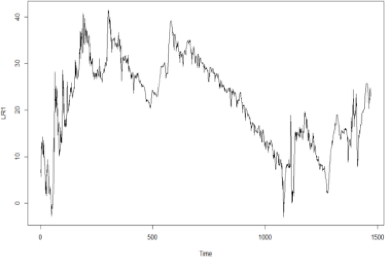
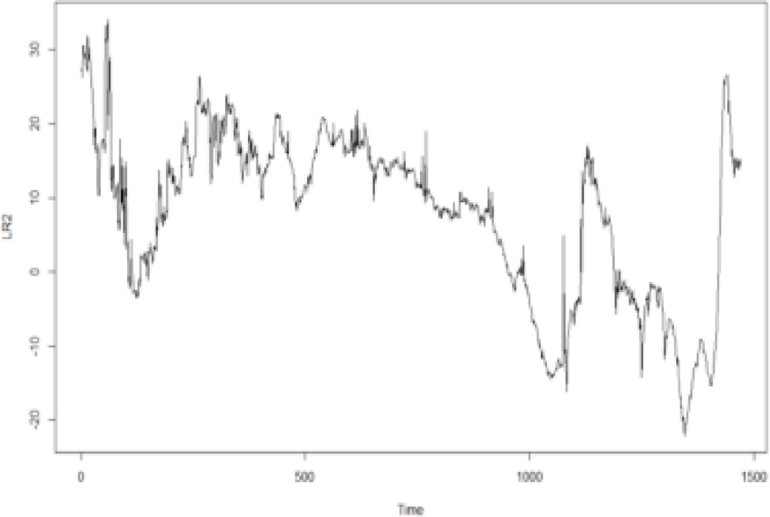
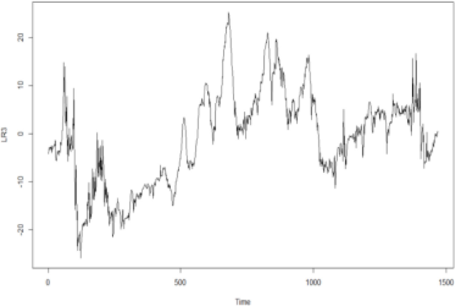
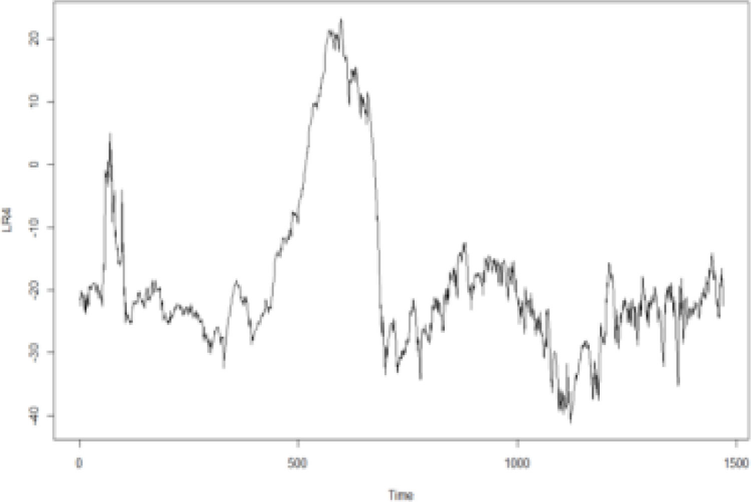
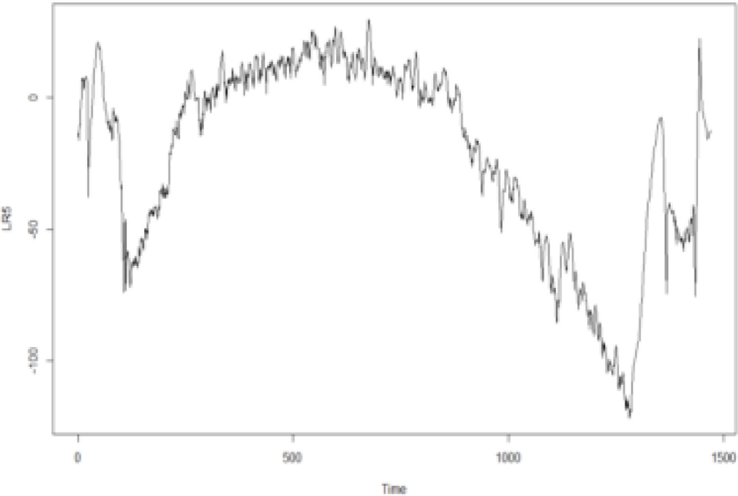
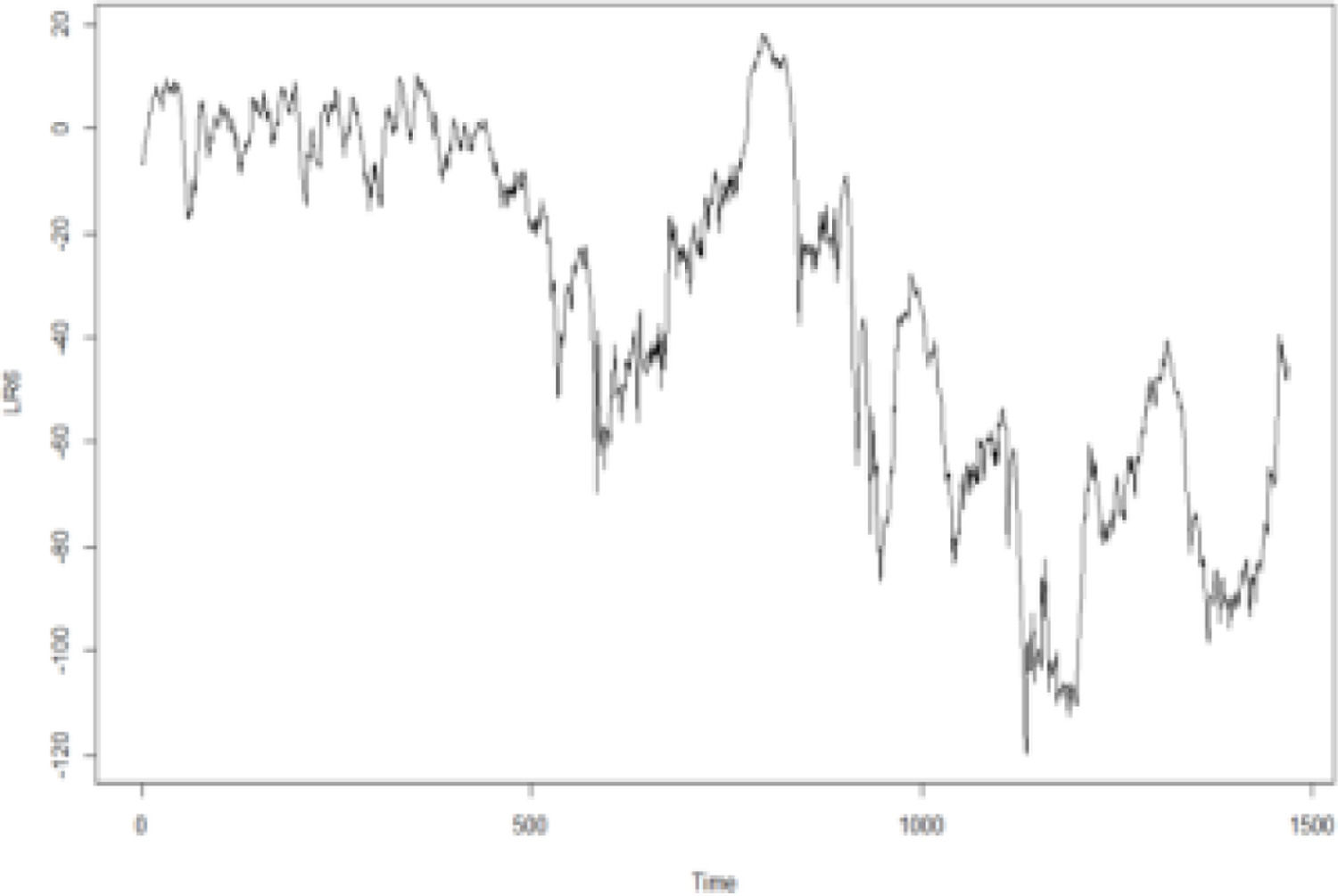
In addition, according to the Kendall rank correlation coefficients in Table 3, there is a positive relationship between the international crude oil and nonferrous metal market. International crude oil shows the closest relationship with copper markets, followed by the aluminum, lead, zinc, tin, and nickel markets. Since the change points in the connections between the international crude oil and the six nonferrous metal markets are unknown, this study adopts the GJR-GARCH-copula to examine the dynamic connection between the two markets. Specifically, the maximum likelihood of the copula function is used to detect change points. Figs. 1-6 show the time series figures of LRk of six nonferrous metal markets.
In Figs. 1-6, the statistics LRk and the corresponding change points between crude oil and each nonferrous metal market can be found. The change points are the times of the potential structural changes Table 4. lists the potential times corresponding to the change points of the connection between the crude oil and nonferrous metal market.
From Figs. 1-6 and Table 4, it can be seen that the structural change in the crude oil and copper markets occurred in 2016; that in the aluminum market occurred in June 2015. This change point may be affected by the production policy of the Organization of Petroleum Exporting Countries (OPEC). Since 2015, major changes have occurred in the oil and gas markets both locally and abroad. Because it was affected by the shale gas revolution in the United States, OPEC adopted a strategy of maintaining market share in 2014 and insisted on the position and policy of non-reducing production. This has led to a continued oversupply of the international oil and gas market. International oil and gas prices have continued to fall since 2014, and this situation continued until 2016. The lowest price of Brent crude oil futures at the beginning of this year was $27 per barrel. Although the demand in the crude oil market rebounded slightly in 2016, the elasticity of the supply side was relatively large. Global oil and gas investment began to decline. Subsequently, OPEC also took measures, such as joint production restrictions, to raise oil and gas prices; the effect was significantly lower than expected. Changes in the international oil and gas market have had a great impact on the supply and demand of the Chinese oil and gas market.
Structural changes in crude oil and lead, zinc, tin, and nickel occurred mainly from the second half of 2017 to the first half of 2018. From 2014 to 2016, international oil and gas prices continued to be sluggish. Since OPEC announced the implementation of the production reduction agreement in December 2016, international oil prices rose significantly in 2017, and the supply and demand patterns of the world oil market improved. In this context, the OPEC and 10 non-OPEC oil-producing countries headed by Russia once again decided to extend the production reduction agreement until the end of 2018. As of December 11, 2017, the price of Brent crude oil futures was approaching $65 per barrel, and the oil market was once again boosted. This agreement has since achieved remarkable results.
From the change points in Table 4, we can see the dynamic connection and discover the nature of its dynamic development, but the purpose is to forecast returns. The occurrence of these change points indicates that the connection experienced essential changes during this period. The connection in the early period makes little contribution to forecast returns, whereas the useful information for forecasting is the connections starting from the nearest change point. In fact, the information before the change will cover useful information, resulting in inaccurate knowledge about dynamic connections. This is the formation of good knowledge about dynamic connections, which is confirmed by the accuracy of the return forecasts.
Return forecast resultsThis section divides the total sample of 1466 into two parts: the "estimated sample" and the "forecast sample". Monte Carlo and rolling simulations are used to calculate the VaR between the two markets. To illustrate the accuracy of the VaRs, this study analyzes both the descriptive statistics of the VaRs and test results. The results are compared with the VaRs predicted by the full-sample data.
Because VaR measures the maximum possible loss value at a higher confidence level, the VaRs in Figs. 7-12 are almost all below the returns. VaR values decrease as the confidence level increases. The change trends of VaR based on the subsample from the post-change point and the full sample are consistent with actual returns. This shows that both samples can accurately describe the connections between crude oil and the six nonferrous metal markets; therefore they can forecast VaRs.
The backtesting resultsTo examine the prediction of VaRs from different sample data, this study analyzes the VaR backtesting results and compares the accuracy of VaRs based on full-sample data and subsample data using the unconditional coverage test. The results are presented in Table 5.
Return test results of VaR value in different markets.
It can be seen from Table 5 that, for different markets, the backtesting results of VaRs all accept the null hypotheses in Eq. (13) or (14) based on two different samples at the 95%, 97.5%, and 99% confidence levels, indicating that the VaRs under the two sample data are relatively accurate.
Although the VaR values all pass the backtesting based on sample data from the post-change point and the full-sample data, there is a large difference between the test values under the two different sample data. The p values corresponding to the VaRs based on sample data from the post-change point are all greater than those based on the full-sample data at different confidence levels in all markets, except for the crude oil-copper market at the 97.5% confidence level. This suggests that the test results based on sample data from the post-change point are more likely to accept the null hypothesis. Therefore, it can be considered that compared with the risk measured under the full-sample data, the structural change points found by data driving can avoid subjectivity partitioning. In addition, the accuracy of return forecasts based on sample data from the post-change point is attributed to the exact establishment of the dynamic connection between crude oil and nonferrous metal market.
ConclusionThis study aims to provide good knowledge about the dynamic connection that favors the accuracy of return forecasts. We construct a nonlinear dynamic connection to explain the relationship between international crude oil and China's nonferrous metal market. Further, we examine the role of dynamic connections in forecasting the returns of the two markets. The empirical results are as follows.
We develop a change-point detection copula method to explore the dynamic connection between international crude oil and China's nonferrous metal market, which can reveal the structural break characteristics of the connection. The results show that a dynamic connection exists between crude oil and nonferrous metal market. We can observe the dynamic connection and discover its dynamic nature.
However, it is remarkable that dynamic connection has an impact on forecasting returns. The p values corresponding to the VaRs based on sample data from the post-change point are all greater than those based on the full-sample data at different confidence levels in all markets. The accuracy of return forecasts based on sample data from the post-change point is attributed to the exact establishment of the dynamic connection between crude oil and nonferrous metal market.
The dynamic connection is related to the production policy of the Organization of Petroleum Exporting Countries (OPEC), which spurs the occurrence of change points. This suggests that the dynamic connection between international crude oil and China's nonferrous metal market fails to be characterized well by any specific copula, which should be divided by change points. The dynamic connection between their prices cannot be ignored. In fact, the information about connection before the change points may have a negative impact on the real connection due to useful information being covered. The “good knowledge” about the dynamic connection is developed by the information from the nearest change point, rather than all the information in the whole process. Our results also show that returns are forecast accurately based on “good knowledge” about the dynamic connection.
As an important strategic resource in China, the price fluctuation of crude oil will affect the prices of other important energy sources such as nonferrous metals. Our good knowledge reveals the dynamic connection between the international crude oil and China's nonferrous metal market, which is helpful to further explore the prices fluctuation law of nonferrous metals in China. This is conducive to accurate returns forecasting, thereby promoting financial stability and healthy development. However, there remain many perspectives on the connection between the international crude oil and nonferrous metal market. In future work, there are still many issues worthy of in-depth investigation. Metrics such as CoVaR can be used to measure the risk spillover effects of international crude oil and nonferrous metal markets to provide more comprehensive information to decision makers and market participants.


