Impact of the stock market capitalization and the banking spread in growth and development in Latin American: A panel data estimation with System GMM

Abstract

This research is aimed at assessing the impact of the stock market capitalization and the banking spread in per capita economic growth (as a proxy of economic development) in the major Latin American economies during period 1994–2012. To do this, a panel data model is estimated with both system and difference Generalized Method of Moments. The main empirical findings are that economic growth in the countries under study is positively impacted by the stock market capitalization and negatively by the banking spread. Typical problems of multicollinearity and autocorrelation appearing in panel data analysis are corrected under the proposed methodology.

Resumen

Esta investigación tiene como objetivo evaluar el impacto de la capitalización de mercado de valores y el spread bancario en el crecimiento económico per cápita (como proxy del desarrollo económico) en las principales economías de América Latina durante el período 1994-2012. Para ello, se estima un modelo de datos de panel con el Método Generalizado de Momentos tanto en sistema como en diferencias. Los principales hallazgos empíricos son que el crecimiento económico en los países estudiados es afectado positivamente por la capitalización bursátil y negativamente por el spread bancario. Los problemas típicos de multicolinealidad y autocorrelación que aparece en el análisis de datos de panel son corregidos bajo la metodología propuesta.

Introduction

There are many investigations, both theoretical and empirical, examining the impact of the financial sector in economic growth. One of the pioneer papers that emphasize the role of the financial sector in the dynamism of the economy is that of Wicksell (1934). He finds the following features: 1) the banking system determines the interest rate in the credit market, 2) the banking system controls the supply of credits through the emission of secondary currency, and 3) credit demand is an engine of growth. Moreover, Wicksell states that the interest rate in the credit market is smaller than the natural rate of interest; in this manner, employers expect their income rise above their costs. Therefore, employers extend their production, which, in turn, lead to competition for factors of production and, consequently, to a more dynamic economy.

Added to previous discussion, Schumpeter (1954) argues that credit demand boosts the economy. Schumpeter states that the financial sector plays a crucial role in financing investment, innovation and technological progress, and, in this sense, the financial sector contributes to economic growth. In this regard, Goldsmith (1969) finds a positive relationship between financial development and economic growth through a cross-cutting analysis for a sample of 35 countries.

On the other hand, Levine (1991) states that financial markets contribute to economic growth through the stock market, which facilitates long-term investment, helping with this to reduce risk and, simultaneously, enabling liquidity to savers, as well as providing a permanent financing to companies. Levine and Zervos (1998) also highlight that there is a significant number of empirical studies supporting the existence of a relationship between capital markets and economic growth in the long run. In this sense, the capital market is a key factor in economic growth, as it channels funds for new investments stimulating an increase in production.

Among the authors considering the financial sector as an important factor for economic growth it can be mentioned, for example: McKinon (1973), King and Levine (1993), Bencivenga, Smith, and Starr (1996), Rajan and Zingales (1998), Beck and Levine (2002), and Hernandez and Parro (2004). Most of them find a positive relationship between the development of the financial sector and economic activity. In this research, the impact of the financial sector in GDP per capita (as a proxy of economic development) in major economies in Latin America is assessed. The variables of the financial sector that will be analized, in this investigation, to examine their impact on the growth rate of real GDP per capita in 1994–2012, are: market capitalization of the firms listed on the stock exchange, market capitalization of the companies listed on the stock exchange as a proportion of GDP, banking spread, and domestic credit provided by the banking sector as a share of GDP. To accomplish this, an analysis of dynamic panel data with information from the World Bank will be carried out. Finally, on the basis of the proposed econometric model, this research provides a number of recommendations that could increase welfare levels in the region.

Referring to the available literature in the subject matter, this work distinguishes in the following: 1) it focuses on Latin America emphasizing the seven major economies (Argentina, Brazil, Chile, Colombia, Mexico, Peru and Venezuela); 2) it has a greater availability of data regarding the past; 3) it carries out an analysis of static and dynamic panel data that allows a greater number of countries and periods in which variables are defined; and 4) it corrects problems of multicollinearity and autocorrelation.

The rest of the paper is organized as follows: section 2 deals with a literature review on the subject matter; section 3 determines, through a theoretical model, the growth of Total Factor Productivity (TFP), that is, the component of output growth that is not explained by capital and labor, for instance, financial factors; section 4 carries out a graphical descriptive analysis of the relevant variables; section 5 deals with some technical issues of the analysis of panel data regarding the model specification; section 6 presents the discussion of the obtained empirical results of the studied countries; and, finally, section 7 provides the conclusions and several policy recommendations.

Financial sector and economic growth

Contrasting with the main visions of endogenous growth driven by Romer (1986), Lucas (1988), and Aghion and Howitt (1992) that have gained much attention, respectively, on technological knowledge, human capital, and industrial innovation to explain technological progress and output growth¹, and the issue of the impact of the financial sector and its effect on economic activity has had less attention than it deserves. Fortunately, the research concerned with the link between the performance of financial markets and economic activity has restarted again showing important theoretical and empirical advancement. In this regard, it is wortth pointing out the work from: King and Levine (1993), De Gregorio (1996), De la Fuente and Marín (1996), Rajan and Zingales (1998), Levine and Zervos (1998), De Gregorio and Kim (2000), Levine, Loayza, and Beck (2000), Morales (2003), Levine (2004), Ang and McKibbin (2007), Pholphirul (2008) and Greenwood, Sanchez, and Wang (2010). Most of these studies suggest that financial development positively affects economic growth.

It is commonly stated that the financial sector promotes economic growth by increasing the rate of capital accumulation and improving the efficiency. In this respect, King and Levine (1993) analyze a sample of 80 countries and found, in most cases, that the financial sector improves economic efficiency and it is correlated with the per capita GDP growth. Moreover, De Gregorio (1996) studies credit constraints that increase aggregate savings, which, in turn, contributes to economic growth. De Gregorio also argues that credit constraints have negative effects on human capital accumulation and, hence, on output growth.

In the empirical literature on the subject, it can be found strong empirical evidence that the development of the financial sector encourages innovation accelerating technological progress, which leads to economic growth. In this regard, De la Fuente and Marín (1996) analyze the interaction of financial intermediaries, physical capital accumulation, technological progress and economic growth. They argue that economic growth is based on the development of new varieties of intermediate goods. They also point out that the probability of success of an innovation depends on the actions of both entrepreneurs and financial intermediaries. The latter negotiate contracts with innovators allowing a better distribution of risk and a higher level of innovative activity, accelerating technological progress and economic growth. These authors conclude that financial intermediaries channel savings to more productive investment projects, identifying the best entrepreneurs and the best technologies, reducing the risks associated with innovation, and contributing to economic efficiency, technological progress and economic growth.

The development of the financial sector plays an important role in relaxing the restrictions on external financing of firms and, hence, in promoting economic growth. In this regard, Rajan and Zingales (1998) study a sample of 36 industries belonging to 48 countries, and conclude that the development of the financial sector drives economic activity. They noticed that the financial system helps mobilize savings and allocate capital contributing to economic activity. The empirical evidence presented by Levine and Zervos (1998) also suggests that the development of the stock market is positively correlated with economic growth in the long term.

There is also empirical evidence that the financial sector can promote the accumulation of human capital. In this regard, De Gregorio and Kim (2000) present a model of endogenous growth in which credit markets affect the distribution, in time, of people with different educational abilities. In this way, the specialization in work can increase growth and welfare. These authors also discuss the relevance of the opening of the credit markets and its effect on income distribution, as well as the importance of intergenerational savings to cover the absence of credit markets.

On the other hand, Levine et al. (2000) analyzed a sample of 77 countries and found that causality makes sense from financial development to economic growth. Moreover, these authors found a positive relationship between financial development and economic growth in the long term; however, in countries where there have been financial crises it remains a negative short-term relationship. The operation of the financial system and economic growth is also analyzed by Levine (2004). This author studies the causality between financial sector and economic activity. Levine also finds that more developed financial systems help reduce external financial constraints faced by firms; being this the mechanism through which financial development influences economic growth.

Greenwood et al. (2010) develop a model of financial intermediation. They use cross-sectional data of interest-rate differentials and per capita GDP. Their analysis suggests that a country like Uganda could increase its production by 116 percent if it had adopted best practices in the financial sector worldwide.

Furthermore, Rodríguez-Benavides and López-Herrera (2009) studied the relationship of financial development on economic growth in Mexico after reforms of the financial sector in 1990. They estimated a dynamic aggregate production function and found a positive impact of financial development on economic growth in Mexico during the period 1990–2004. Cermeño and Roa (2013) provided an assessment of recent theoretical and empirical literature on the effects of financial development on economic growth by analyzing the interaction channels between these variables. They found that most of the research asserts that financial development positively affects economic growth.

Recently, Mhadhbi (2014) reviews the empirical relationship between financial development and economic growth by using data from developed and developing countries in the period 1973–2012. He uses a panel data model and finds that the banking system availability influences economic growth with a significant and positive impact. On the other hand, he finds that the loans granted by the financial system to the private sector have a negative influence on growth, while financial deepening of the economy seems to depend positively on economic growth for developing countries and negatively by developed. Rashti, Araghi, and Shayeste (2014) studies the influence of financial development on economic growth with emphasis on the recent financial crisis in the United States in 2008. They find that the recent financial crisis had different effects depending on the country. They results from the estimated models show that the financial crisis had the greatest influence in developing countries with high average income that in developed countries and developing countries with low and middle income. They also find that capital markets have shown positive effects on economic growth in countries with low average incomes and a negative effect on high- and middle-income developed countries during 1990–2010.

Statistical description of the variables

The data used in this research was obtained from the World Bank. The period of analysis is 1994–2012. The dependent variable is GDP per capita (as a proxy of economic development) at constant prices of 2005. The independent variables are: the stock market capitalization of the firms listed on the Stock Exchange (in U.S. dollars at current prices), the market capitalization of the listed companies as a percentage of GDP, the banking spread (lending rate minus deposit rate), and the domestic credit provided by the banking sector as a percentage of GDP. This research utilizes balanced panel data and the period is restricted to the availability of data. The panel data analysis includes the seven larger Latin American economies in the period 1994–2012. The notation for the main variables and their statistics are presented in Table 1.²

Table 1.

Statistics of the variables under study.

Variable	Notation	Average	Deviations	Minimum	Maximum
GDP per capita	gdpper	5271.17	2853.86	1509.19	14 501.25
Stock market capitalization in USD	capiusd	1.58E+11	2.63E+11	3.66E+09	1.55E+12
Stock market capitalization as a proportion of GDP	capigdp	40.23137	33.29331	33.29331	157.1864
Banking spread	difi	13.10239	13.44323	1.390658	58.36
Domestic credit provided by banking sector as a proportion of GDP	credipsbgdp	45.08259	24.44503	10.51353	110.5377

Source: Data from World Bank.

Table 1 shows the averages, deviations, and maximum and minimum levels of the variables under study. For the sample of the seven countries, the average GDP per capita is 5271.17 USD, the standard deviation is 2853.86 USD with a minimum of 1509.19 and a maximum of 14 501.25 USD. The average value of the capitalization market is 40.23% of GDP, the standard deviation of GDP is 33.29%, the minimum of GDP is 33.29% and the maximum of GDP is 157.18%. With respect to the interest rate differential, the average is 13.10%, the deviation is 13.44%, with a minimum of 1.39% and a maximum of 58.36%. The credit provided by the banking sector as a proportion of GDP on average is 45.08%, with a deviation of 24.44%, a minimum of 10.51% and a maximum of 110.53%.

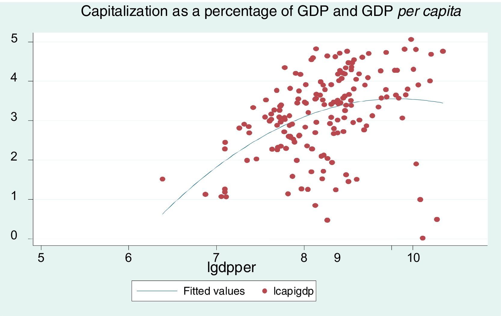
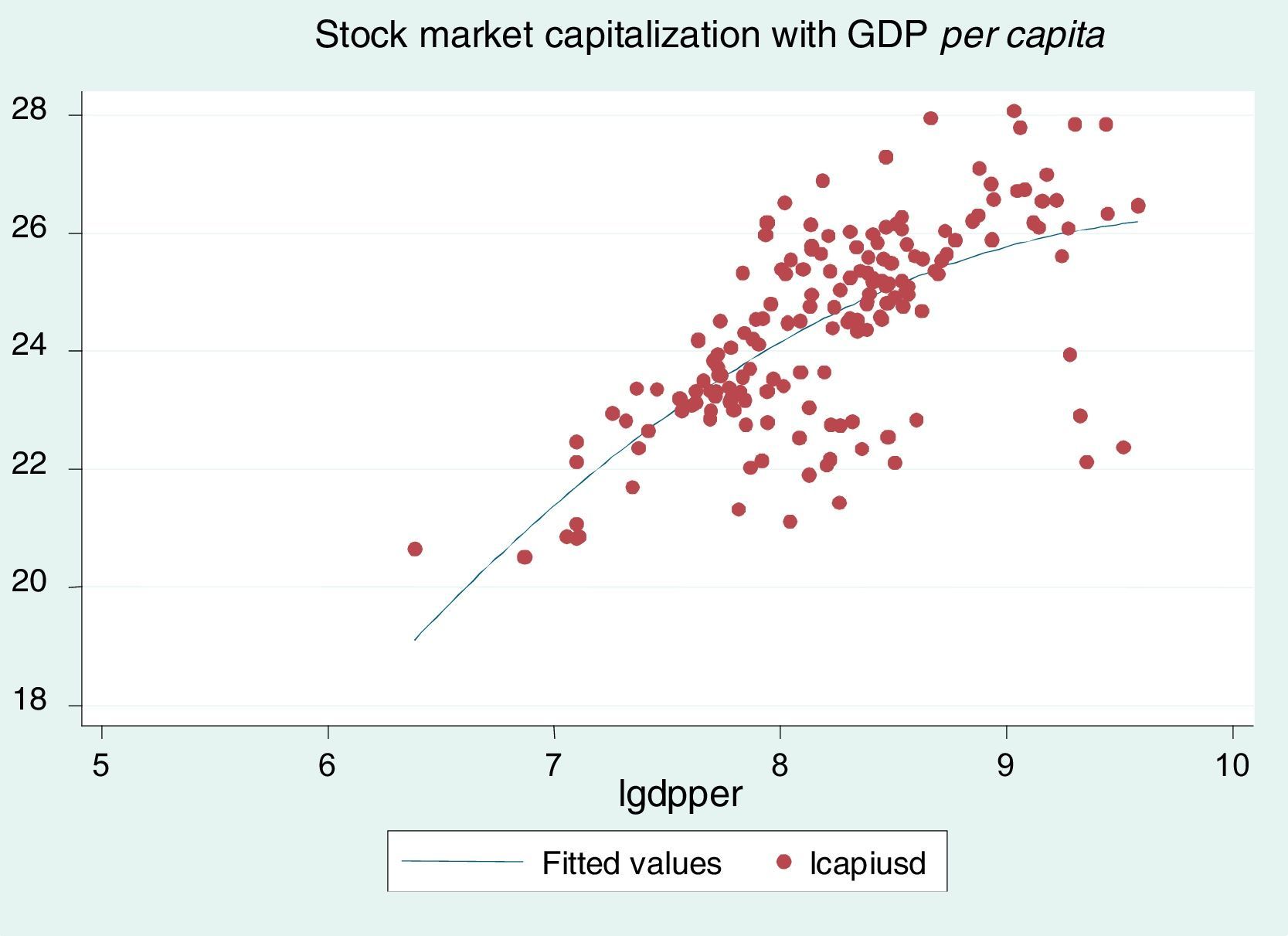
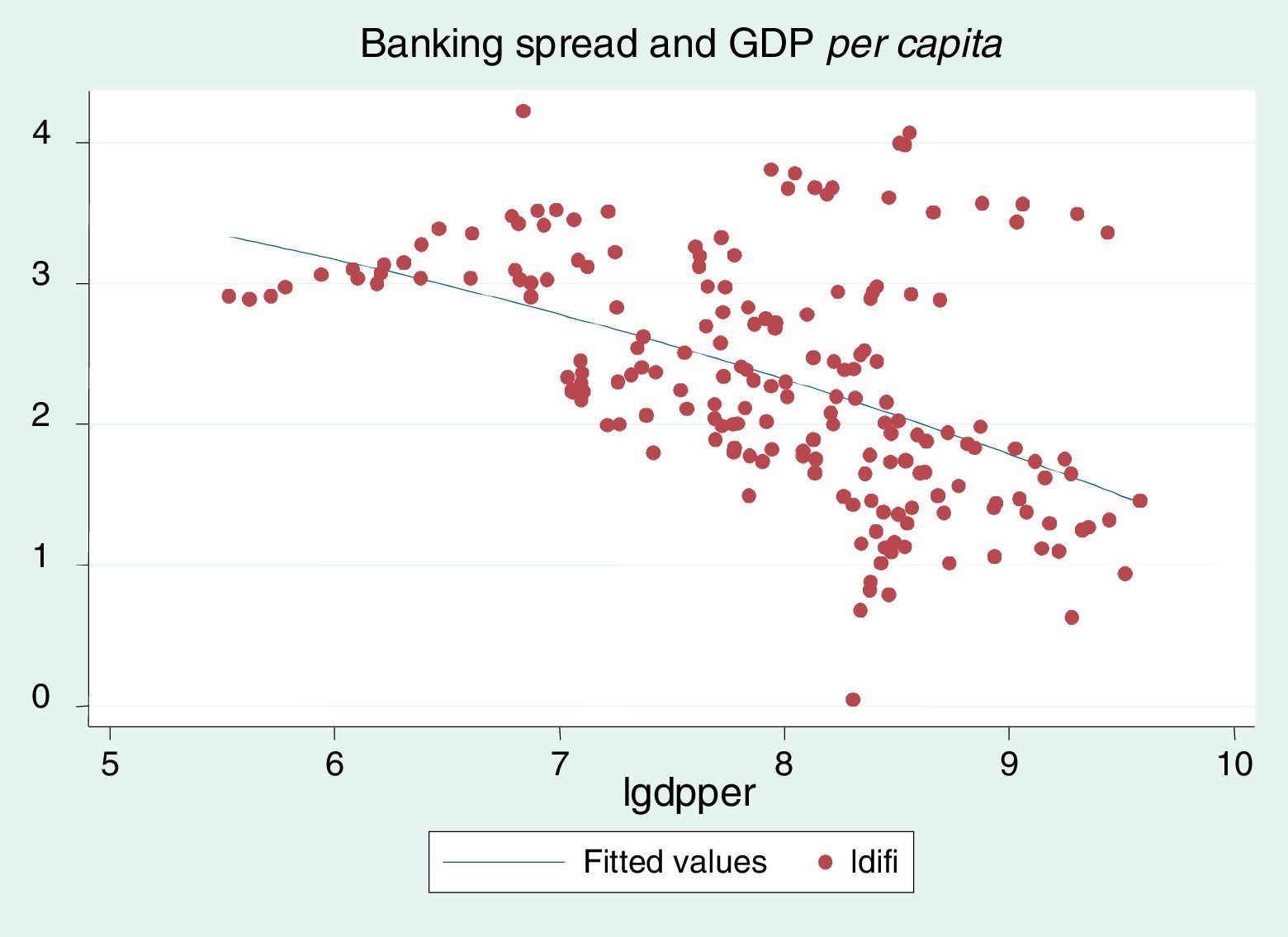
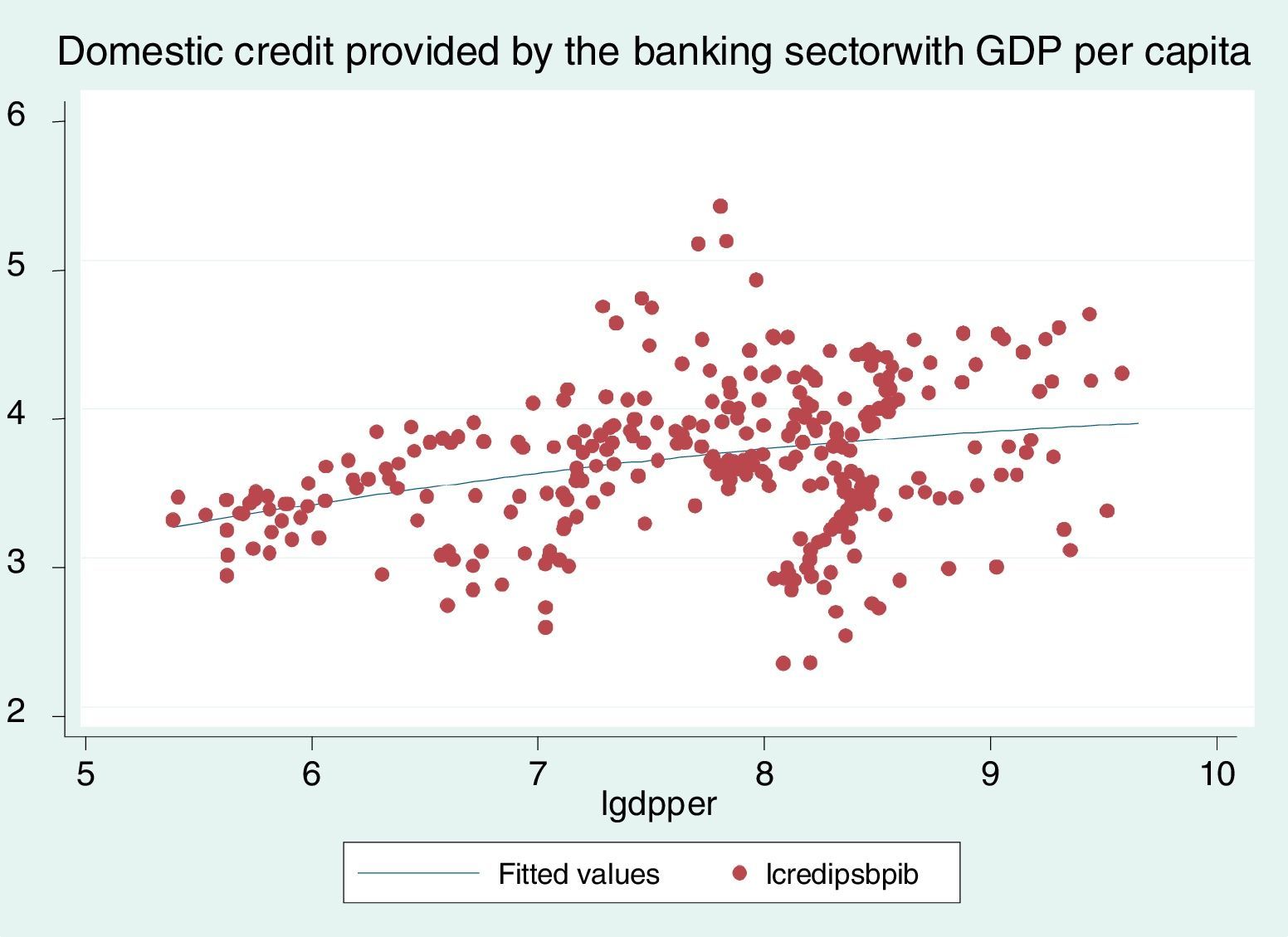
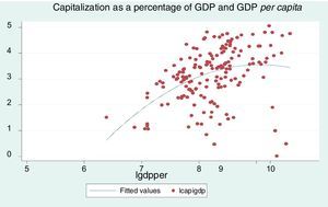
As discussed before, most of the research concerned with examining the relationship between expansion of the financial sector and economic growth predicts a positive correlation between them. The following graphical statistical analysis, showed through Figs. 1–4, reinforces this argument.

Fig. 1.

Capitalization as a percentage of GDP and GDP per capita.

Source: Data from World Bank.

Fig. 2.

Stock market capitalization with GDP per capita.

Source: Data from World Bank.

Fig. 3.

Banking spread and GDP per capita.

Source: Data from World Bank.

Fig. 4.

Domestic credit provided by the banking sector with GDP per capita.

Source: Data from World Bank.

Fig. 1 shows the behavior of the stock market capitalization as a percentage of GDP and its relation to per capita GDP for the seven analyzed economies. It can be observed a positive correlation between these variables, indicating that the increase in the capitalization value of listed companies as a percentage of GDP leads to an increase in GDP per capita, i.e., a higher level of stock issuers as a proportion of GDP tends to increase GDP per capita, and, therefore, raises economic development.

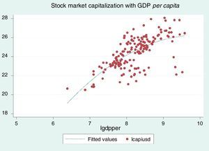
Fig. 2 shows a positive relationship between stock market capitalization in USD and per capita real GDP. The chart indicates that a greater volume of stock of listed companies tends to increase GDP per capita. In other words, if the financial sector develops and capitalizes larger volumes, then there is a positive impact on the increase in per capita output.

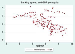
Fig. 3 shows the differential of interest rate (lending rate minus deposit rate) and its relation to GDP per capita for the set economies in this study. A negative relationship (which is expected) between the banking spread and GDP per capita is found. That is, an increase in the banking spread declines gross domestic product per capita.

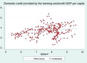
Finally, Fig. 4 shows that an increase in domestic credit provided by the banking sector as a share of GDP tends to increase GDP per capita. All the above graphs support, again, the argument that financial sector expansion leads to economic growth. In the sequel, we will be concerned with finding more robust empirical evidence through a panel data analysis that a larger capitalization value of companies listed in the stock exchange as a proportion of GDP and a lower differential in banking interest rates are both positively related with an increase in GDP per capita.

Analysis of panel data

The use of panel data analysis is becoming more common in econometric research since it is very valuable for comparing the performance of units (countries). In our approach, panel data is a combination of time series data and cross-section. The general model to be estimated is expressed as follows:

where y_it is the dependent variable that changes depending on i (the countries) and t (the number of years), y_it−1 is the lagged dependent variable, X_it are exogenous variables, and u_it are random perturbations. The estimation of Eq. (1) by ordinary least squares (OLS) is usually biased. To avoid this limitation there are alternative models dealing with pooled regression that nest data by incorporating fixed effects (FE) and random effects (RE), which will be discussed forward.

The use of panel data has several benefits since it allows examining a larger number of observations with more and heterogenous information. It also supports a larger number of variables, and produces less data multicollinearity among the explanatory variables. Another benefit is that it allows using more data and can keep track of each unit of observation. The problem of omitted variables is partially removed because differences can eliminate variables that do not change over time.³ As expected, the panel data analysis has also disadvantages as the data become more complex and heterogeneity appears and is not properly treated. If the qualities of the country are not observable, then the errors will be correlated with the observations, and the OLS estimators are inconsistent. Subsequently, the fixed effects model will be introduced. This involves fewer assumptions about the behavior of residuals and the equation to be estimated is given by:

It is supposed in this case that εit=vi+uit, hence

The error ¿_it can be decomposed into two parts: a fixed part that remains constant for each country vi, and a random part u_it that meets the requirements of OLS (εit=vi+uit), which is equivalent to performing a general regression and giving each individual a different point source (ordinate).

The random effects model (RE) has the same specification as the fixed effects except that the term v_i, rather than being fixed for each country and constant over time is a random variable with mean Evi and variance Var(v_i) ≠ 0. Thus, the model is given by:

where now v_i is a random term. The RE model is more efficient but less consistent than FE. For the estimation of the dynamic panel data, we will be using the Generalized Method of Moments (GMM); see, for example, Arellano and Bond (1991). The difference GMM estimator developed by Arellano and Bover (1995) is based on difference regressions to control unobservable effects. Subsequently, they use previous observations of explanatory variables and lags of the dependent variables as instruments.

The difference GMM estimator has disadvantages and limitations as shown by Blundell and Bond (1998), particularly when the explanatory variables are persistent over time. In this case, lagged values of these variables are weak instruments for the difference equation. Moreover, this approach biases the parameters if the lagged variable (in this case, the instrument) is very close to being persistent. To deal with this drawback, these authors propose the introduction of new moments on the correlation of the lagged variable and the error term. To do this, the conditions of covariance between the lagged dependent variable and the difference of the errors as well as the change in the lagged dependent variable are added; the level of the error must be zero. The system GMM estimation uses a set of difference equations which are instrumented with lags of the equations in levels. This estimator also relates a set of equations in instrumented levels with lags of difference equations (Bond, 2002).

The system GMM estimator includes sufficient orthogonality conditions that are imposed to ensure consistent estimates of the parameter even with endogeneity and not observed individual-country effects. This approach will be used to estimate the parameters and was developed by Arellano and Bover (1995), several improvements were made later by Blundell and Bond (1998). The estimator thus obtained has advantages over the FE estimators and others, and it does not produce biased estimators of the parameters in small samples or in the presence of endogeneity. In this case, the GMM optimal estimator has the following form:

This equation is a system consisting of a regression containing information jointly in levels and in differences in terms of moment conditions:

The above relations will be applied to the first stage of the system. The regression in differences and time conditions, which are written below are applied to the second stage, that is, in a regression in levels:

Under this approach, the lags of the variables in levels are used as instruments in the regression in differences, and only the most recent differences are used as instruments in the regression in levels. The model generates consistent and efficient estimated coefficients, and also provides information on differences such that:

The error component vi* proceeds from both models, both levels as differences, which can be defined as:

The array of instruments for difference GMM includes information on the explanatory variables and the lag of the dependent variable:

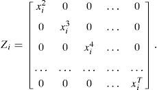
while the matrix of instruments for the equation in levels only enter the explanatory variables without the lagged dependent variable

The instrumental matrix takes the following form and is included in the GMM estimator:

Finally, the matrix V_N is the covariance matrix of the valid time constraints for the optimal case:

Additional tests to ensure the smooth running of GMM are suggested by Arellano Bond autocorrelation tests of first and second orders, and the Sargan test of overidentifying in considering the following statistic:

This statistic of test has a χ²-distribution where vˆ is the vector of residuals, Z the number of conditions imposed, k the number of parameters included in the vector β, and p is the number of columns of the matrix Z. The Sargan test examines the overall validity of the instruments analyzed. Subsequently, the existence of second-order serial correlation of the differentiated error term, which has to be normally distributed, is reviewed.

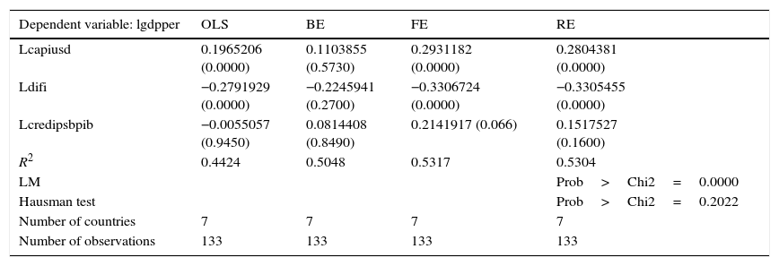
Analysis of empirical results

The purpose of this section is to specify a panel data model that properly allows studying the relationships between the financial sector and the growth of GDP per capita focusing on a sample of the seven largest Latin American economies: Argentina, Brazil, Chile, Colombia, Mexico, Peru and Venezuela. The analyzed variables are expressed in logarithms: “lpibper” stands for the logarithm of GDP per capita real, “lcapiusd” is log-capitalization companies traded in USD, “lcapipib” represents the logarithm of the capitalization of listed companies as a proportion of gross domestic product, “ldifi” is the logarithm of the interest rate differential, and “lcredipsbpib” is the logarithm of credit provided by the banking sector as a proportion of gross domestic product. The period analyzed is 1994–2012, which allows for a total of 133 observations from 7 groups. A balanced panel model will be estimated with the econometric package Stata.11. The main results are shown in Table 2.

Table 2.

Estimates of static panel data.

Dependent variable: lgdpper	OLS	BE	FE	RE
Lcapiusd	0.1965206 (0.0000)	0.1103855 (0.5730)	0.2931182 (0.0000)	0.2804381 (0.0000)
Ldifi	−0.2791929 (0.0000)	−0.2245941 (0.2700)	−0.3306724 (0.0000)	−0.3305455 (0.0000)
Lcredipsbpib	−0.0055057 (0.9450)	0.0814408 (0.8490)	0.2141917 (0.066)	0.1517527 (0.1600)
R^2	0.4424	0.5048	0.5317	0.5304
LM				Prob > Chi2 = 0.0000
Hausman test				Prob > Chi2 = 0.2022
Number of countries	7	7	7	7
Number of observations	133	133	133	133

The corresponding standard errors are in brackets.

Source: Data from the World Bank.

Table 2 shows the results of four static estimates of panel data. The first column indicates that the dependent variable is the logarithm of GDP per capita as stated before. The explanatory variables are the logarithm of the market capitalization of listed companies in USD, the logarithm of the interest rate differential, and the logarithm of the credit provided by the banking sector as a proportion of GDP. Notice that the logarithm of the market capitalization of listed companies as a proportion of GDP does not have the expected sign and it is not significant in all estimation methods, thus it will not be included in the subsequent models. For all the models the coefficient of determination are calculated and the Lagrange multiplier and Hausman tests are performed. The second column shows the OLS estimate of the logarithm of the market capitalization of listed companies, which results positive and significant. The logarithm of the differential interest rates has also the expected negative sign and is significant. The logarithm of the credit provided by banks as a share of GDP is negative not having the expected sign, and is not significant either. It is important to note that, in this case, R² is 0.4424. The third column of Table 2 shows the results of the Between (BE) estimates, in which all variables in the financial sector have the right sign, but they all are not significant, and in this case the value of R² is 0.5048. The fourth column presents the estimation results with FE, all coefficients have the appropriate signs and are significant, though the coefficients of “lcredipsbpib is not significant at the 5% level; here R² is 0.5317. The last column shows the results of the estimation RE indicating appropriate signs and significant coefficients for the logarithm of the market capitalization of listed companies in USD and the logarithm of the interest rate differential. The log ratio of credit provided by the banking sector as a proportion of GDP has the right sign but is not significant, the R² is 0.5304. The Lagrange multiplier test yields prob > chi2 = 0.0000, which indicates that the random effects estimation is preferable to ordinary least squares. Finally, Hausman test provides prob > chi2 = 0.2022 indicating that the estimation RE is preferable to FE. In summary, the estimates for the four static panel data methods, i.e., OLS, “between”, fixed and random effects, and the evidence of Lagrange Multiplier and Hausman tests indicate that the RE estimation is preferred to explain the impact of the financial sector in economic growth. However, when performing complementary tests, autocorrelation problems are detected since prob > chi2 = 0.0382, and Durbin Watson = 0.514. This shows that the null hypothesis of no autocorrelation can be rejected, which corroborates autocorrelation. To solve the autocorrelation problem, several models of dynamic panel data are estimated with the Generalized Method of Moments (GMM). The main results of the estimation of dynamic panel data are presented in Table 3.

Table 3.

Estimates of dynamic panel data with system GMM.

Dependent variable: lpibper	GMM differences (one step)	GMM differences (two steps)	GMM system (one step)	GMM system (two step)
Lgdpper.L1	0.9129491 (0.000)	1.147017 (0.191)	0.9075942 (0.000)	0.9177252 (0.000)
Lcapiusd	0.0720906 (0.000)	−0.0821172 (0.877)	–	–
Ldifi	−0.0405024 (0.237)	0.0163088 (0.929)	−0.0855443 (0.000)	0.0142242 (0.904)
Lcredipsbpib	−0.0595762 (0.298)	−0.0111214 (0.973)	–	–
Lcapiusd.L1	–	–	0.0423051 (0.002)	0.0287133 (0.276)
AR(1) Prob > Z =	0.000	0.2285	0.000	0.020
AR(2) Prob > Z =	0.214	0.9774	0.734	0.785
Sargan Test Prob > Chi2 =	0.091	1.00	0.472	0.001
Hansen Test Prob > Chi2 =	–	–	–	1.000
Number of countries	7	7	7	7
Number of observations	119	119	126	126

The corresponding standard errors are in brackets.

Source: Based on data from the World Bank.

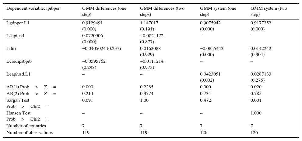
Table 3 shows the results of the estimates of dynamic panel data. The first column indicates that the dependent variable is the logarithm of GDP per capita real, and the explanatory variables are: the lag of log GDP per capita real, the logarithm of the market capitalization of listed companies in USD, the logarithm of the interest rate differential, the logarithm of the credit provided by the banking sector as a proportion of GDP, and the lag of the logarithm of the capitalization of the companies listed in USD. The second column of the above table shows the results of the estimation by difference GMM in one step. The coefficients have the expected signs, excepting the log of credit provided by the banking sector as a proportion of GDP (lcredipsbpib). While the coefficients of the lag of GDP per capita “lpibper.L1” and “lcapiusd” are significant, it turns out to be that “ldifi, credipsbpib” is not. Also, the first-order serial autocorrelation is not rejected, but the second-order autocorrelation is rejected. The Sargan test does not reject the null hypothesis, therefore the model specification is not supporting the general validity of the instruments. The third column shows the results of the estimation by difference GMM in two stages. All coefficients are not significant, and the lagged dependent variable has the correct sign while the rest of the explanatory variables do not exhibit the proper sign. Both the first-order and the second-order serial autocorrelation are rejected. In the Sargan test the null hypothesis is not rejected, therefore the model specification and the overall validity of the instruments are supported. The fourth column presents estimates by system GMM in one stage, all coefficients of the explanatory variables have the right signs and are significant, and the first order autocorrelation is not rejected, but the second-order autocorrelation is rejected. The Sargan test admits the correct specification of the model and the overall validity of the instruments. The system GMM estimates in one stage is preferred and more suitable than the previous ones. Therefore, this could be the model to be chosen to explain the impact of the financial sector in economic growth. The fifth column presents estimates for system GMM in two stages. In this case, the coefficient of the lagged dependent variable “lpibper.L1” has the right sign and is significant, while the coefficient of “ldifi” do not have the proper sign and it is not significant. The coefficient of the lagged logarithm of the market capitalization of listed companies “lcapiusd.L1” presents the appropriate sign, but it is not significant. On the other hand, the first-order autocorrelation is not rejected, but the second-order autocorrelation is rejected. The Sargan test indicates an incorrect specification of the model and the Hansen test points to the appropriate use of the methodology. Estimates indicate that the best fitting model is the system GMM in one step, indicating that the per capita GDP is positively related to GDP per capita (lpibper.L1), GDP per capita is also positively related to the delay of the capitalization of the companies listed, and GDP per capita this negatively related to the interest rate differential. The estimated system GMM in one stage indicates that an increase of 1% of the capitalization of listed companies in the past year will have a 4% impact on GDP per capita in the current year, while an increase 1% in the interest rate differential will cause a decline about 8% of GDP per capita.

Conclusions

The empirical evidence presented in this study shows that the financial sector is relevant and has important effects on economic growth and development. Therefore, a major effort in the expansion of the financial sector will help boost economic activity in Latin America resulting in a higher welfare level of the population.

This research also has shown that an increase in the capitalization of listed companies, an increase of the domestic credit provided by the banking sector, and a declining in interest rate differentials have a positive relationship with per capita income, thereby in economic development in Latin American. The panel data dynamic estimations showed the importance of financial variables to economic and development growth. It is worth pointing out that the delayed impact of the capitalization of the listed companies promotes per capita GDP, and a higher impact of the reduction in the interest rate differential raises per capita GDP.

From this research some recommendations are derived for Latin American countries. The countries should look for tools and incentives to promote a higher capitalization of the listed companies, and look for reducing the interest rate differential to promote the expansion of the financial sector. This will contribute to higher levels of economic growth and population welfare. Finally, the expansion of the financial sector in Latin America should be a key objective for policy and decision makers to encourage economic development.