A Multi-Product Lot-Sizing Model for a Manufacturing Company

Abstract

This paper presents an Integer Linear Programming model for a multi-product lot-sizing problem. The problem considers demands, inventory policies, backorder costs and the search of an efficient use of resources (machines and workers). The real-world case used to illustrate the model is from a Colombian company, which produces raw material for the bakery industry. The short term planning for the company under study is critical, because there is a multi-product environment whit shared resources by different products and processes. The computational experiments show the effectiveness of the proposed model.

Resumen

Este artículo presenta un modelo de programación entera para un problema de tamaño de lote con múltiples productos. El problema considera demandas, políticas de inventario, costos de pedido y la búsqueda del uso eficiente de recursos (máquinas y trabajadores). El caso real que se utilizó para ilustrar el modelo es de una compañía colombiana, la cual produce materias primas para la industria de la panadería. La planeación a corto plazo para la compañía bajo estudio es crítica, debido a que existe un ambiente de multiproductos con recursos compartidos por diferentes productos y procesos. Los experimentos computacionales muestran la efectividad del modelo propuesto.

Introduction

The manufacturing operations planning in the short term field is a widely studied area. There are many cases of research projects by considering the specific characteristics of a particular manufacturing system. These studies try to represent real-world cases offering support for future decision-making processes. The definition of lot-sizing problem (LSP) considers features and decision variables from the production and inventory control area, and their impact on the service level. Usually, the objective function for the LSP is to minimize the sum of the total holding costs, of the stock-out costs, and of the other costs which affect the operation of each system (Robinson et al., 2009; Jans and Degraeve, 2007).

In particular, our problem considers several characteristics increasing the complexity of the traditional LSP. In this work, the proposed integer lineal programming model (ILP) considers a given planning time horizon, number of levels, number of products, several patterns of demand, holding inventory, back- orders, and setups structures. Karimi et al. (2003) propose a general classification about the most frequent issues to consider in a lot-sizing problem. Different models by including one item for incapacitated and capacitated versions of the LSP have been proposed in Brahimi et al. (2006). In particular, these models consider one product, few production stages, and known demands.

Aksen et al. (2003) introduce the concept of immediate lost sales by considering inventory policies for a single product; while Absi and Kedad (2008) consider inventory policies for a multi-item capacitated model by adding setup times. Robinson et al. (2009); Jans and Degraeve (2007), introduce three important concepts about inventory management: stock out, back-orders and holding costs. All of these approaches consider a dynamic demand environment.

Capacity constraints and relaxed demand constraints with a penalty are considered in Aksen (2007). This relaxation includes variables to represent back-orders and inventory levels among different periods. Other mathematical approaches can be found in Abad (2000). Toro et al. (2009) and Kovacs et al. (2009) propose set of constraints and variables to represent the multiple stage condition for the LSP. In these works, a new concept is introduced: scheduling with sequence-dependent setups. All conditions previously presented increase computational complexity with a major computational effort. Heuristic approaches for the LSP are proposed by Xie and Dong (2002) and Minner (2009).

A production program in a multi-product environment must consider three fundamental aspects:

• i)

  the type of products to schedule,

• ii)

  the amount of products to produce,

• iii)

  the time to make the products.

The first aspect is generally solved by giving priority to an item close to stock out or to reorder point. The other two aspects are closely related, if small batches are scheduled. The way of scheduling lots, their sizes, and their frequencies, are the main causes of the final performance for the objective function. Setting larger lots imply a greater efficiency, but also imply more scheduling time for a single product at a given time. This decision could affect the responsiveness of the system.

In this paper, the considered real-world case has a batch system for the production of a bakery industry. Currently, different dry products (dough improvers, premixes, and sugar among others), and a wide range of liquid essences are produced. In general, these products represent about seventy different references with approximately two thousand tons annually. In addition, a two-stage multi-product environment with deterministic demands allowing back-orders and holding inventory is considered. Due to similarity inside each family of products, setups are considered as constants with an independent sequence.

Mathematical model

Let us introduce the following notation for the proposed ILP model:

Sets

• •

  set of products indexed by i, where i = 1,…, I

• •

  set of shifts indexed by j, where j = 1, …, J

• •

  set of days indexed by k, where k = 1, …, K

• •

  set of machines indexed by m, where m = 1, …, M

Subsets

• •

  subset of production machines indexed by m, where m ∈ α ⊆ M

• •

  subset of packing machines indexed by m, where m ∈ β ⊆ M

• •

  subset of products with a production stage indexed by i, where i ∈ μ ⊆; I

• •

  subset of products with production and packing stage indexed by i, where i ∈ θ ⊆ I

Parameters

H_im

required time to produce one kilogram of each product i at machine m (hr/kg)v

p_m

hard-work force required per shift at machine m (number of persons)

MO

total persons available

RP_i

maximum requirement of product i (kg)

IS_i

initial stock of product i (kg)

RD_ik

daily requirement of product i at day k (kg/day)

CI_i

holding cost of product i ($/kg-day)

CB_i

backorder cost of product i ($/kg-day)

CH_m

overtime cost at machine m ($/hr)

HM

maximum overtime (hr)

HT

time available per shift (hr/shift)

A

setup time (hours/setup)

TML_i

minimum lot-size of product i (kg)

Decision variables

x_ijkm

amount of product i scheduled in shift j of day k at machine m (kg)

y_jkm

1 if shift j is scheduled in day k at machine m, 0 otherwise

he_jkm

overtime in shift j in day k at machine m (hr)

f_ik

backorder of product i in day k (kg)

s_ik

inventory of product i in day k (kg)

wip_ik

work in process of product i in day k (kg)

w_ijkm

1 if product i is scheduled in shift j in day k at machine m, 0 otherwise

Objective function

The performance of the system is defined by three different sets of costs: holding costs, backorder costs, and overtime costs. The first set (holding costs) is related to the operations required to control and manage items, and to the financial value of investment in products, work in process and raw materials. The second set (backorder costs) is associated to the decreasing value defined by the final customer. Finally, the third set (overtime costs) is considered as a linear ratio which represents additional time for each machine. The objective function corresponds to the minimization of the equation (1):

Constraints

Constraints (2) ensure that the number of persons in each shift for each machine must not exceed the total available hard-work force.

Constraints (3) limit the production capacity. The maximum capacity is expressed as the sums of the time available for each scheduled HT, and of the overtime, minus the sum of the setup time employed by each assigned product. These constraints are considered as production efficiency if the size of the programmed batch is larger, and the number of setups is smaller.

Constraints (4) add overtime according to the maximum number of possible hours.

Constraints (5), (6) and (7) make logical relations between shift programming and scheduled products during the available shifts by considering lot-size (which is set within the range [TML_i, RP_i]), and setup time for each product.

Constraints (8) include back-orders and inventory control to keep inventory balance among days. The basic expression considered here is initial stock + productionrequired product = final inventory. The final inventory is shown as a linear combination of f_ik and s_ik. Indeed, only one of these set of variables will be activated each time, because the cost in the objective function.

Finally, the multi-period issue is restricted in (9). The final inventory for a given period k-1 is calculated.

Equations (10) and (11), represent the condition expressed in (9) for products belonging to the subset θ

Products θ have two stage processes, which must be connected to ensure process flow and work in process. Constraints (12) described the first period, and constraints (12) described the multi-period stage.

Constraints (14) are the non-negativity constraints.

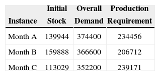
Computational results

Scenarios

Three different instances were selected to represent the behavior of the system and the relations between variables, constraints and parameters in the proposed model. These scenarios have different demands, initial stocks and production requirements. Table 1 shows the information of the initial stock, the overall demand, and the production requirement used by Instances.

Table 1.

Instances features (kg)

	Initial	Overall	Production
Instance	Stock	Demand	Requirement
Month A	139944	374400	234456
Month B	159888	366600	206712
Month C	113029	352200	239171

Each scenario has different characteristics and different production requirements. Consequently, the computing time and the function objective value will be different.

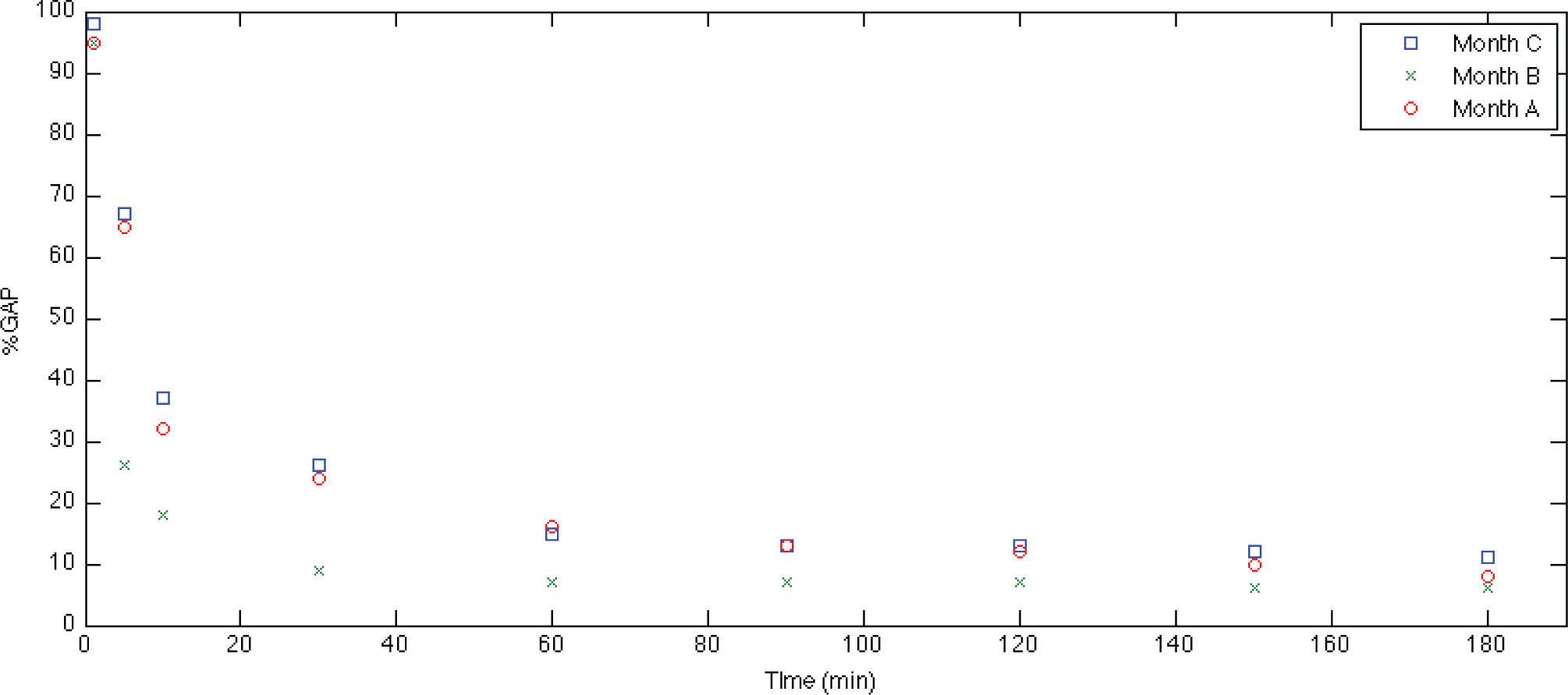
Global results

The tests were carried out by using CPLEX 12.3 on an Intel Core i5 2.3 GHz processor with 4 GB of memory. In the used real-world case, the computing time of the proposed model is relevant, in order to be considered as support decisions tool for a short period term. Indeed, computing time must be efficient according to the planning horizon. Figure 1 shows the results of the used computing time to find the optimal solution. The behavior for months A and C are similar respect to the computing time. It can be inferred by the fact of the relations with the total number of kilograms used by the company. In the case of month B, the computing time is smaller because the amount is only almost by thirty tons.

Figure 1.

Evolution to reach optimal solution

The proposed instances consider seventy products, five work stations, three shifts, and a planning horizon of twenty four days.

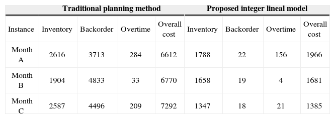
Performance of the objective function

Table 2 details the costs obtained for each instance. We have compared the final results with the traditional planning method used by the company. It is worth to note that the proposed model outperforms the currently planning method respect to the overall cost. Indeed, the main reductions of the costs occur in backorder cost and inventory cost.

Table 2.

Comparison of the performance for each ingredient of the objective function (thousand $)

	Traditional planning method				Proposed integer lineal model
Instance	Inventory	Backorder	Overtime	Overall cost	Inventory	Backorder	Overtime	Overall cost
Month A	2616	3713	284	6612	1788	22	156	1966
Month B	1904	4833	33	6770	1658	19	4	1681
Month C	2587	4496	209	7292	1347	18	21	1385

Lot size

The lot size is a significant issue related to the efficiency and the cost of the production program. In a multi-product environment, a big lot size for a given product can delay the production of the other products. This situation is consequence of the shared resources (machines and hard-work force). In the previously traditional planning method, the considered lots had an average of two thousand kilograms. The proposed ILP model is able to find a more equitable replenishment of the different products. Smaller lots are found as described Table 3. In this table, the following notation is used: Average is the average size of the lots, STD is the standard deviation for scheduled lots, Q1 is the first quartile (lowest 25% of lots), Q2 is the second quartile (data set in half), and Q3 is the third quartile, lowest 75%.

Table 3.

Lot size (kg)

Instance	Average	STD	Q1	Q2	Q3
Month A	1311	982	630	996	1714
Month B	1091	776	600	768	1222
Month C	1178	792	600	810	1500

The obtained lot sizes consider less than 1700 kg. Indeed, this lot size permits to produce many products frequently keeping healthy stocks levels, and avoiding stock-outs.

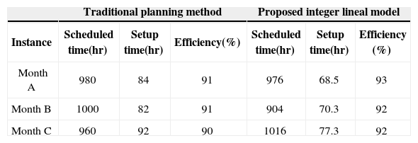
Efficiency analysis

We have added some new variables and constraints to the proposed ILP model. These variables and constraints allow estimating other performance measures. The variables at represent the scheduled time and variables st represent the total time spent during setups.

Table 4 presents the results obtained by the efficiency of the ILP model for the three months. Indeed, Table 4 shows scheduled time, setup time, and efficiency.

Table 4.

Comparison of efficiency performance

	Traditional planning method			Proposed integer lineal model
Instance	Scheduled time(hr)	Setup time(hr)	Efficiency(%)	Scheduled time(hr)	Setup time(hr)	Efficiency (%)
Month A	980	84	91	976	68.5	93
Month B	1000	82	91	904	70.3	92
Month C	960	92	90	1016	77.3	92

The results of the proposed ILP model are slightly better than those proposed by the traditional planning method. In the traditional planning method bigger lots are chosen, so the efficiency is increased. Nevertheless, matching the demands of many products for a given month must be changed decreasing the efficiency of the system.

Concluding remarks

We have proposed an effective ILP formulation for a multi-product lot-sizing problem. The results show that ILP model outperforms the traditional planning method used by the real-world company. The objective function considers holding costs, backorder costs, and overtime costs. This approximation allows establishing requirements without additional costs. The minimum lot size and the simultaneity of the requirements for different products are the main conditions to stock a certain amount of inventory.

The total computing time of the proposed ILP model is considerably high because the number of variables and constraints. Moreover, since the multi-product lot-sizing problem is a monthly planning problem, the model is not solved frequently. Therefore, the computing time remains in an acceptable range for a tactical decision like multi-product lot-sizing problem. Additionally, results with a 10% gap respect to the optimal solution can be obtained, within short computing times. These values could be used as an approximation method for production planning by the real-world company.

In a multi-product environment, the size of each batch affects the level of inventory for a given product and the references which use the same resources (persons and machines). In particular, a common aspect is to schedule small batches (values range from a minimum batch operation and 1800 kilograms).

Acknowledgment

The work of the second author has been partially supported by MIUR (Ministero Istruzione, Universitá e Ri-cerca), Italy and Pontificia Universidad Javeriana Cali, Colombia. This support is gratefully acknowledged.