A novel Diamond-Mean predictor for reversible watermarking of images

Abstract

Reversible watermarking (RW) is the art of embedding secret information in the host image such that after extraction of hidden information, original image is also restored from the watermarked image. Prediction error expansion (PEE) is state of the art technique for RW. Performance of PEE methods depends on the predictor's ability to accurately estimate image pixels. In this paper, a novel Diamond-Mean (D-Mean) prediction mechanism is presented. The D-Mean predictor uses only D-4 neighbors of a pixel, i.e. pixels located at {east, west, north, south}. In the estimation process, apart from edge presence, its orientation and sensitivity is also taken into account. In experimental evaluations, the D-Mean predictor outperforms currently in use MED (median edge detector) and GAP (gradient adjusted predictor) predictors. For, standard test images of Lena, Airplane, Barbara and Baboon, an average improvement of 51.79 for mean squared PE and an average improvement of 0.4 for error-entropy than MED/GAP are observed. Payload vs imperceptibility comparison of the method shows promising results.

1

Introduction

Internet is a highly convenient medium for transmitting and sharing of multimedia data. It rejuvenated businesses by attracting large number of customers. With the ease of access and increased business benefits, arises a greater challenge of ownership and authenticity of the media content. Watermarking of multimedia content is a very popular technique of coupling secret information with images and videos.

Image watermarking is the art of hiding ‘secret message’ in the image in such a way that it should not cause any visible distortion. It is one of the recent image protection methods, which provides security against illegal production and re-sharing of the copyright content. The process of hiding secret information is called as ‘watermark embedding’. When an image, also known as ‘cover-image’, undergoes embedding process it is called as ‘watermarked-image’. The main objective of watermarking is to make the watermarked-image alterations imperceptible to the image viewer, i.e. the quality of cover-image and watermarked-image should be visually identical. The amount of data that can be successfully embedded and retrieved in the cover-image is called as ‘payload’ of the embedding method. Increase in payload affects the imperceptibility negatively and vice versa.

Methods that can extract the watermark (hidden message) as well as completely retrieve the cover image from its watermarked-image are called as reversible watermarking (RW) methods (Caldelli, Filippini, & Becarelli, 2010). Recovery of the cover image is very important in medical imaging or in military applications where even a minute alteration/distortion is unacceptable. An MRI or CT scan image of a patient if not fully recovered might endanger the life of a patient by misleading the physician. Other applications of RW include remote sensing (Barni, Bartolini, Cappellini, Magli, & Olmo, 2001) and multimedia archive management (Park, 2014). Many reversible watermarking techniques has been proposed in the most recent literature (Kotvicha, Sanguansat, & Kasemsa, 2012; Shi & Xiao, 2013; Song, Li, Zhao, Hu, & Tu, 2015; Zhang, Qian, Feng, & Ren, 2014; Zhao & Feng, 2016).

Tian (2003) introduced difference expansion transform for RW which was followed by prediction-error expansion (PEE) method by Thodi and Rodríguez (2004, 2007) they introduced histogram-shifting (HS) which significantly reduced location map (LM) size. Since then, many variations of PEE based methods (Kamstra & Heijmans, 2005; Luo, Chen, Chen, Zeng, & Xiong, 2010; Peng, Li, & Yang, 2012; Sachnev, Kim, Nam, Suresh, & Shi, 2009; Tai, Yeh, & Chang, 2009; Wang, Li, & Yang, 2010) were developed. Performance of these methods heavily rely on the predictor's ability to accurately predict image pixels. In most of the methods researchers investigated different embedding mechanisms while not much work is being done in developing new predictors. MED (Weinberger, Seroussi, & Sapiro, 2000) and GAP (Wu & Memon, 1997) are mostly used predictors by these methods.

In this paper a novel predictor for reversible watermarking is proposed. The predictor accurately models the flat and edge regions in an image hence better prediction of pixels which leads to less distortion of watermarked image. Improved embedding of watermark in conjunction with histogram shifting and D-Mean predictor led to gain higher imperceptibility levels for a given payload.

The paper organization is as follows: In the next section relevant reversible image hiding methods are discussed. In Section 3, MED and GAP are reviewed and novel D-Mean predictor is presented. Reversible watermarking method based on the proposed predictor is discussed in Section 4. Experimental setup and results are provided in Section 5 and conclusions are drawn in Section 6.

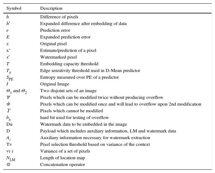
2

Related work

First expansion based method was presented by Tian (2003) and it achieved moderate payload with good image quality. In this method, image is divided into pairs of pixels and each pair based on its mean and difference value undergoes 1 bit of data embedding. Let (x₀, x₁) be the values of a pair of pixels, then integer mean and difference are denoted as l = ⌊(x₀ + x₁)/2⌋ and h = x₁ − x₀. To embed 1 bit watermark b ∈ {0, 1} in h, it is expanded to h′ = 2h + b and watermarked values (x0′,x1′) are obtained using Eq. (1). For an easy reference, notations used in the paper are summarized in Table 1:

Table 1.

Notations.

Symbol	Description
h	Difference of pixels
h′	Expanded difference after embedding of data
e	Prediction error
E	Expanded prediction error
x	Original pixel
xˆ	Estimate/prediction of a pixel
x′	Watermarked pixel
T	Embedding capacity threshold
TS	Edge sensitivity threshold used in D-Mean predictor
SPE	Entropy measured over PE of a predictor
I	Original Image
Θ1 and Θ2	Two disjoint sets of an image
Ψ	Pixels which can be modified twice without producing overflow
Φ	Pixels which can be modified once and will lead to overflow upon 2nd modification
ϒ	Pixels which cannot be modified
bh	hard bit used for testing of overflow
Du	Watermark data to be embedded in the image
D	Payload which includes auxiliary information, LM and watermark data
Ai	Auxiliary information necessary for watermark extraction
Tv	Pixel selection threshold based on variance of the context
v(·)	Variance of a set of pixels
NLM	Length of location map
⊙	Concatenation operator

Pairs which are not suitable for data embedding are listed in location map (LM). For successful extraction of hidden data and restoration of cover image pixels, LM is also stored in the watermarked-image alongside embedded bits as overhead information. Originally, image pixel values range from 0 to 255 for an 8 bits per pixel representation. Expanded pixels which lie outside the permissible range are marked as unexpandable pairs in LM. Size of LM hampers the embedding capacity (EC); therefore reduction in its size is very important, hence researchers are using lossless compression methods to reduce its size. Using Tian method, 1 bit can be embedded in each pair of pixels while 1 bit for each pair is also required in LM hence space for data embedding is created by lossless compression of LM.

Alattar (2004) extended the idea of a pair to k pixels cell. Each cell has been used to hide k − 1 bits. For each cell one bit is required in LM, this helps decrease the size of LM to (1/k)th the image size. Unexpandable cells cannot be used for embedding due to problems of underflow or overflow (noted as overflow), so payload of the method is always less than (k − 1)/k bpp (bits per pixel).

Location map is the bottleneck of reversible image hiding methods. Even compressed LM takes significant part of the payload. Thus, LM size determines the performance of a method. Later, authors investigated methods that generate small-size location map or no map at all. Lee, Yoo, and Kalker (2007) used block-based approach with integer-to-integer wavelet transform to hide data. An image of size X × Y is divided into blocks of size N × M. The method produces relatively small LM and better exploits redundancy present in the sub-bands of wavelet transformed coefficients, hence, outperforms Tian (2003) and Alattar (2004).

Image pixels are highly correlated with neighboring pixels. Thodi and Rodríguez (2004) used MED predictor to predict image pixels from their neighborhood pixels. The prediction error (PE) is used to hide watermark bits instead of difference between pairs of pixels. In prediction, more than one pixel of the neighborhood is used which results in smaller PE. PE denoted as e of a pixel x having prediction value xˆ, is computed using Eq. (2). In Thodi and Rodríguez (2007), HS was incorporated in error expansion. In this method e is expanded for data embedding and the expanded error E is computed using Eq. (3):

Watermarked pixel x′ is calculated using Eq. (4)

In the decoder, E and e are computed using Eqs. (5) and (6) respectively:

Embedded data bit b can be extracted using Eq. (7) and original pixel value is restored using Eq. (8):

Kim, Sachnev, Shi, Nam, and Choo (2008) further used a simplified approach to reduce the size of LM and need for lossless compression was evaded. van der Veen, Bruekers, van Leest, and Cavin (2003) used companding technique for reversible watermarking of audio streams while van Leest, van der Veen, and Bruekers (2004) extended the same method for images. For data hiding Ni, Shi, Ansari, and Su (2006) used shifting of bins in histogram of image pixels. Yang, Schmucker, Funk, Busch, and Sun (2004) presented a generalized RW method for coefficients of integer discrete cosine transform. In another research Yang, Schmucker, Busch, Niu, and Sun (2005), they also used high frequency wavelet coefficients with histogram expansion. Luo et al. (2010) introduced an interpolation based RW method which has high fidelity but with relatively low capacity. Hong, Chen, Chang, and Shiu (2010) presented a high performance error expansion based RW method. Tsai, Hu, and Yeh (2009) compute the residual image from basic pixels and reference pixels in nonoverlapping blocks, high payload is achieved by multilevel embedding in residual image. Luo et al. (2010) used full context for interpolation of a pixel, interpolation error is expanded to embed data. Due to the fact that they have used 8 neighbors of a pixel context their results are significantly improved from methods that uses MED and GAP based prediction mechanism which use 3 and 7 pixels respectively.

Wang, Li, Yang, and Guo (2010) presented generalized version of the Tian's difference expansion algorithm. The difference is converted to extended integer transform and rather than using difference, mean of the block is computed and difference of the mean and pixel is used for embedding. It uses multiple embedding passes to achieve high EC. It had better imperceptibility performance than its predecessors. Hu, Lee, and Li (2009) proposed a major improvement in DE by incorporating MED and dual expansion. Dual expansion is carried out in two stages. In 1st stage the histogram bin is shifted to the right and in the 2nd stage the bin is slightly shifted back to the left, hence reducing/reversing the distortion caused by 1st stage embedding. The performance was further improved by introducing capacity control mechanism.

Peng et al. (2012) proposed a block based method. The image is first divided into non-overlapping blocks. Embedding capacity of each block is computed by using variance as the capacity control parameter. Variance is inversely proportional to the EC of a block. Location map for each block is computed and compressed using a lossless method. Watermark and LM are embedded into each block to generate watermarked image. This approach has better performance at higher payloads.

In most of the expansion based methods MED and GAP predictors are used. As these predictors were designed for lossless compression rather than data hiding, they cannot fully exploit existing correlations among image pixels for the purpose of watermarking.

3

Diamond-Mean predictor

In reversible watermarking methods PE histogram is modeled by Laplacian distribution. This is because of the spatial redundancy in image pixels. To get higher peaks in the center of the PE histogram, high performance predictors are being used in the prediction process. MED (Weinberger et al., 2000) and GAP (Wu & Memon, 1997) are the advanced predictors used in JPEG-LS and Context-based Adaptive Lossless Image Coding (CALIC). In the proposed reversible watermarking method D-Mean (Diamond-Mean) predictor is used. Before presenting the D-Mean predictor MED and GAP are reviewed.

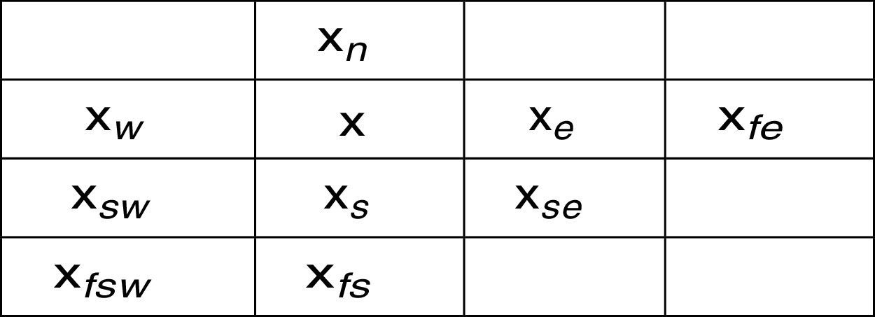
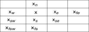
3.1

Median edge detector

MED is one of the mostly used predictor in lossless compression and reversible watermarking. To calculate the prediction it uses forward context pixels. Pixel context is given in Fig. 1. Using MED, the estimate of a pixel xˆ can be calculated using Eq. (9):

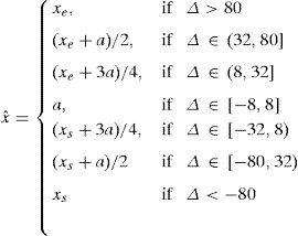
The predictor selects x_s incase a vertical edge is detected, x_e incase of a horizontal edge and x_s + x_e − x_se when no edge is detected. In Martucci (1990) they have denoted it as the median of the set {x_s, x_e, x_s + x_e − x_se}. MED is being used by Thodi and Rodríguez (2007) and many other PE techniques. It efficiently detects the presence of an edge but major limitation is its inability to detect intensity of the edge.

Fig. 1.

Context of a pixel x for MED, GAP and D-Mean predictors.

3.2

Gradient adjusted predictor

GAP is more complex than MED. The prediction context is extended to 7 pixels. It not only detects the existence of an edge but also the intensity (weak, normal, strong). The direction of edge is detected by comparing local gradients with empirical thresholds. It performs better than MED at the expense of mathematical complexity. Estimate xˆ of a pixel is calculated using Eq. (10):

where

Both MED and GAP were originally designed for predictive coding in image/video compression. Due to limitations in coding for compression in the respective standards these predictors only use one side of a pixel context hence are unable to fully exploit the correlation between neighboring pixels.

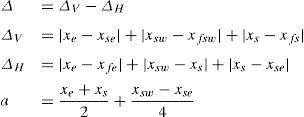
3.3

Proposed Diamond-Mean predictor

A predictor that would better exploit correlation of pixels is presented. The proposed D-Mean (Diamond-Mean predictor) calculates the estimate xˆ=⌊α⌋, while α is calculated using Eq. (11):

where

Set A consists of four neighbors of a pixel, i.e. {xe,xw,xn,xs} as defined in Fig. 1. A′ contains the 2nd and 3rd largest elements of A. M function computes the mean of a set while ⌊α⌋ returns floor of α, i.e. the largest integer less than α.

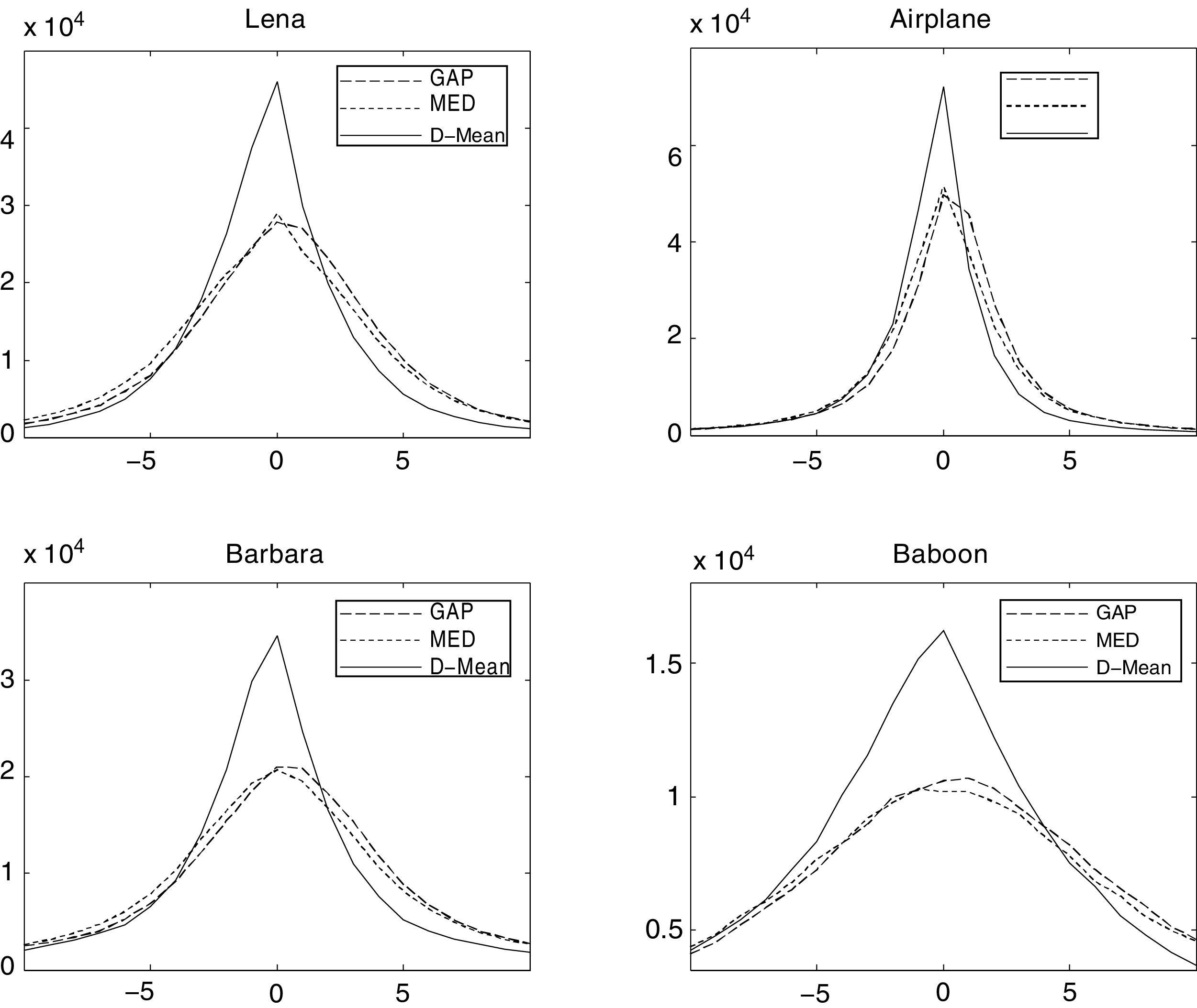
For each pixel, the predictor first checks if neighboring pixels (x_n, x_s) or (xe,xw) are close enough to be on the same edge, an edge sensitivity threshold T_S is used for this purpose. For vertical edges, if both x_n and x_s are less than Min_H (a dark edge on a bright background) or both are greater than Max_H (bright edge on a dark background) then there exist an edge which passes through x_n and x_s (a vertical edge). Horizontal edges are detected in the same manner and current pixel prediction is calculated. If there exist no definite edge, mean of 2nd and 3rd largest pixels from {xe,xw,xn,xs} is taken as prediction. Using this method the predicted value may not be an integer, which must be converted to an integer if it is to be used in RW, for that purpose floor of the predicted value is calculated. The PE histogram of MED, GAP and D-Mean predictors is compared in Fig. 2. Significant improvement is observed for all four standard images, i.e. Lena, Airplane, Barbara and Baboon. Surge in the histogram peaks at 0 and short tail of PE for D-Mean confirms the superior performance of the proposed D-Mean predictor over MED and GAP methods.

Fig. 2.

Prediction-error histograms on standard images. X-axis and y-axis represent PE and its occurrence respectively.

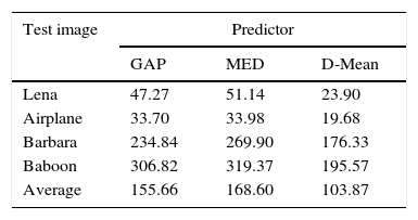
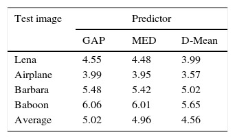
Quantitative measures of predictor's performance are mean squared prediction error (MSPE) and entropy of PE (S_PE). Watermarking method's performance is inversely proportional to both the measures, i.e. smaller MSPE and entropy of PE (S_PE) leads to better imperceptibility results. MSPE is computed using Eq. (12) and S_PE using Eq. (13). Here, e is PE computed using Eq. (2), N_e is the length of error vector, and pr(e) is the probability of error, e. In Table 2, predictors are compared on the basis of MSPE. For all the test images D-Mean yields the least MSPE than MED and GAP. Entropy comparison of PE is provided in Table 3 and again D-Mean has outperformed other predictors. Overall, average performance of D-Mean is also better for both MSPE and S_PE:

Table 2.

Comparison of predictors based on MSPE for standard images.

Test image	Predictor
	GAP	MED	D-Mean
Lena	47.27	51.14	23.90
Airplane	33.70	33.98	19.68
Barbara	234.84	269.90	176.33
Baboon	306.82	319.37	195.57
Average	155.66	168.60	103.87

Table 3.

Comparison based on entropy of the PE, S_PE.

Test image	Predictor
	GAP	MED	D-Mean
Lena	4.55	4.48	3.99
Airplane	3.99	3.95	3.57
Barbara	5.48	5.42	5.02
Baboon	6.06	6.01	5.65
Average	5.02	4.96	4.56

With D-Mean predictor two-stage image traversal mechanism is used. Pixels classification into 2 sets is provided in Fig. 3. Pixels of an image I having positions (i, j) are assigned to disjoint sets Θ₁ and Θ₂. As both sets are disjoint, pixels in Θ₁ can be used in estimation of pixels in Θ₂ and vice versa.

Fig. 3.

Notation of pixels in two disjoint sets where • ∈ Θ₁ and ∘ ∈ Θ₂.

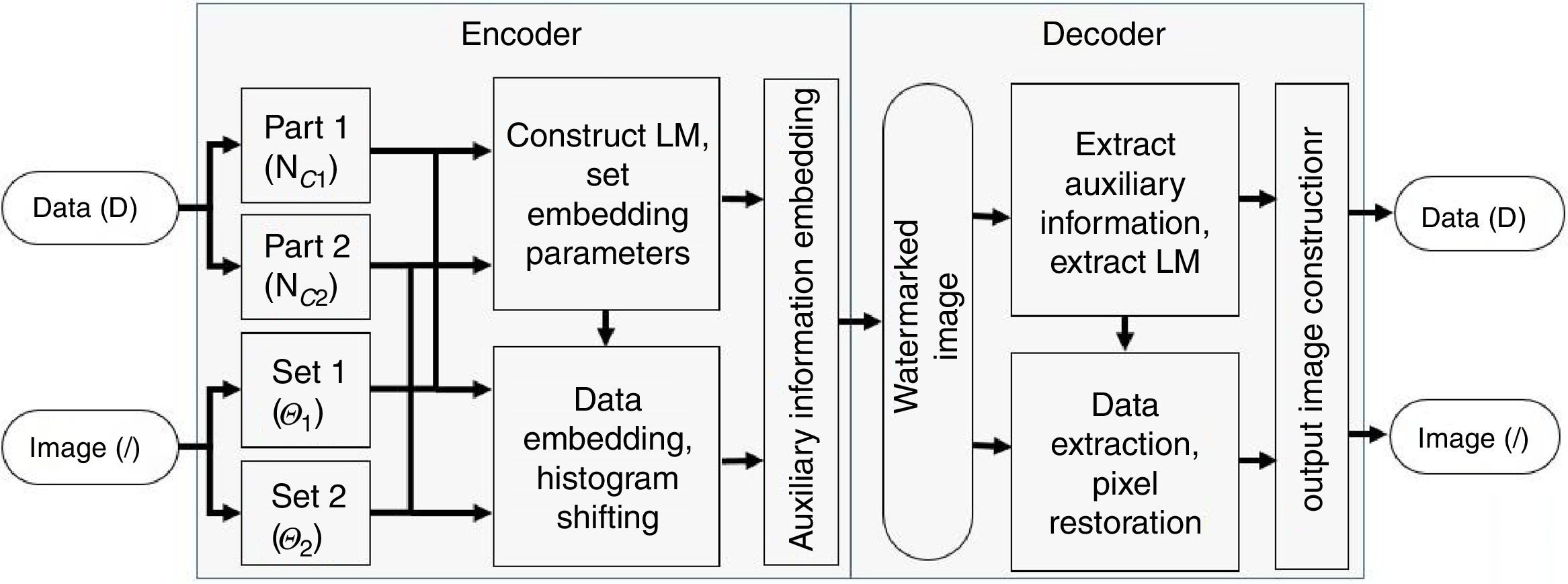
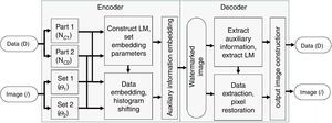
4

Proposed method

Proposed watermarking method uses high performance D-Mean prediction mechanism. Pixel's PE is expanded to embed watermark bits. Some of the pixels that may result in overflow due to embedding are left unmodified in the watermarked image. Intelligent embedding is being used to only select pixels that have small PE which further improved imperceptibility of the proposed method. Illustration of the proposed method is provided in Fig. 4.

Fig. 4.

System block diagram.

Given an image I of size M × N having pixels {(i, j)|1 ≤ i ≤ M, 1 ≤ j ≤ N} is processed in two stages. Θ₁ pixels are processed first. Based on pixel's modifiability 3 sets of pixels are defined for Θ₁, unambiguously modifiable (noted as Ψ), ambiguously modifiable (noted as Φ) and non-modifiable (noted as ϒ) pixels. Pixel's PE is calculated using Eq. (2) and tested by modification with hard bit (b_h) using Eq. (3), modified pixel x^t₁ is calculated using Eq. (4). If x^t₁ satisfies (x^t₁ < 0 ∨255 < x^t₁) it is assigned to ϒ otherwise x^t₁ is further checked for modification with b_h in the same manner and modified pixel x^t₂ is calculated. If x^t₂ satisfies (x^t₂ < 0 ∨255 < x^t₂) it is assigned to Φ, otherwise it is assigned to Ψ. In Eq. (3), b_h is being used for overflow checking in place of b and is defined as:

LM is maintained for pixels that may result in overflow due to embedding. Here an approach similar to Kim et al. (2008), is being used in recording of LM. Pixels in Ψ can be unambiguously interpreted in the decoder, hence these pixels do not require the use of LM. Pixels of the set Φ are only modified with hard bit and pixels of the set ϒ are not modified at all. In LM Φ and ϒ pixels are noted 0 and 1 respectively. In our case LM is a 1D binary string and its length is defined as |Φ| + |ϒ|, here |·| is a cardinal number of the set.

Payload of the proposed method is controlled by EC parameter T as used in Eq. (3). Due to iterative nature of existing RW algorithms, selection of T is a computationally expensive task because they had to compress LM for each value of T. We are using a simple methodology to record LM which significantly reduces its size hence compression is not required. A simple procedure to compute T is followed.

Let N_c be the length of data Du to be embedded in the image. In the proposed two stage processing, N_c1 and N_c2 are the sizes of data embedded in stage 1 and 2 respectively. N_c1 and N_c2 are computed as follows:

Auxiliary information A_i is required for successful extraction of watermark in the decoder. A_i is also embedded as part of the payload in the image. |A_i| is 68 bits, 8 for EC threshold T, 24 for pixel selection threshold Tv and 18 for LM length and 18 for last modified pixel position according to ⌈log₂(M × N)⌉ for 512 × 512 size image. For each stage Θ₁ and Θ₂ three sets ϒ(T), Φ(T) and Ψ(T) can be defined for T ∈ {1, 2, …, 255}. Data embedding in each stage is possible subject to Eq.(16). If T which satisfies Eq.(16) then it is not possible to hide data of size N_ci in each stage.

Smallest T for which, |Ψ(T)|≥D is selected as EC threshold.

Maximum data that can be embedded in a single stage is |Ψ|. Let N_ci be the length of data desired to be embedded in each stage. If D<|Ψ| then a subset Ψ_s of pixels can be selected from Ψ for embedding. Error due to embedding of PEE based methods is directly proportional to the magnitude of PE hence Ψ_s must contain pixels having small PE. Here a pixel selection mechanism is defined based on variance of the neighboring pixels. Let Ψ_s be defined as:

Here x_N for a pixel x at location (i, j) is defined as a set, i.e. {(i − 1, j), (i, j − 1), (i, j + 1), (i + 1, j)} also mentioned as xn,xw,xe and x_s of a pixel context in Fig. 1, while υ(x_N) is defined as:

Tv is a threshold for selection of pixels having small PE. In this way, proposed method tends to select the pixels having small error and hence better visual quality of the watermarked image is obtained.

4.1

Watermark embedding

In this sub-section watermark embedding procedure is listed. Step by step description of the proposed method is followed. Embedding data Du is divided into 2 parts, Du1 and Du2 using Eq. (15). Data streams Du1, Du2 contains Du{1⋯Nc1} and Du{Nc1+1⋯Nc} respectively. Du1 is embedded in pixels from Θ₁ while Θ₂ will be embedded with Du2. For each set, Θ₁ and Θ₂, repeat the following steps:

• Step 1:

  Select the EC threshold T, which satisfies Eq. (16).

• Step 2:

  Compute υ for all pixels using Eq. (18) and arrange pixels in increasing magnitude with respect to υ.

• Step 3:

  Skip the initial 68 pixels. Among the remaining, using Eq. (17) select a subset Ψ_s from Ψ.

• Step 4:

  All pixels of the set, Φ will be modified with hard-bit using Eq. (14). Pixels of the set, ϒ will not be modified but noted in LM. In LM Φ and ϒ pixels are noted as ‘0’ and ‘1’ respectively. Size of LM, N_LM will be |Φ(T)| + |ϒ(T)|

• Step 5:

  Collect LSB of initial 68 pixels and construct the payload as Dup=LSB⊙LM⊙Dui. Where ⊙ is a concatenation operator.

• Step 6:

  Each pixel of the set Ψ_s is used to embed 1 data bit from Dup using Eq. (4). Estimate of the pixel, xˆ is computed using proposed D-Mean predictor.

• Step 7:

  Auxiliary information A_i, consists of 68 bits and contains, T, Tv, N_LM and position of the last modified pixel. Replace LSBs of the initial 68 pixels with A_i.

The above steps 1–7 are repeated for each, Θ₁ and Θ₂. In the second stage for the prediction of pixels modified pixels of the set Θ₁ are used.

4.2

Watermark extraction

In the decoder watermarked image is processed in the reverse order. First, pixels of stage-II, Θ₂ are decoded and restored. Then, Θ₁ pixels are processed. Step-by-step procedure of decoding is described as:

• Step 1:

  Extract LSBs of the initial 68 pixels and compute the parameters of T, Tv, and N_LM and location of the last modified pixel.

• Step 2:

  As done in the encoder, compute υ for all pixels using Eq. (18) and arrange pixels in the increasing magnitude with respect to υ.

• Step 3:

  Make a set Ψ_e of pixels having υ

• Step 4:

  Check each pixel of the set Ψ_e for expansion with hard bit, using Eq. (3) and Eq. (4). This step is performed until we reach the last modified pixel of the set.

  • a.

    If the pixel results in overflow, check LM, it belongs to one of the sets, Φ or ϒ. If corresponding bit in the LM is 0, it belongs to the set, Φ. The pixel is restored using the Eqs. (5) and (8). The bit stored in the current pixel is discarded and is not recorded in the data.

  • b.

    If the pixel did not resulted in overflow then stored data bit is extracted and the pixel is restored. The data bit from the pixel is extracted using Eq. (5) and (7) and recorded in the output data. While pixel restoration is carried out using Eq. (8).

• Step 5:

  Restore the LSBs of initial 68 pixels from the extracted data.

After restoration of pixels of Θ₂. The set Θ₁ is processed in the same manner. Data extracted from both the stages is combined to make the extracted message. Block diagram of the embedding and extraction process is provided in the Fig. 4.

5

Experimental results

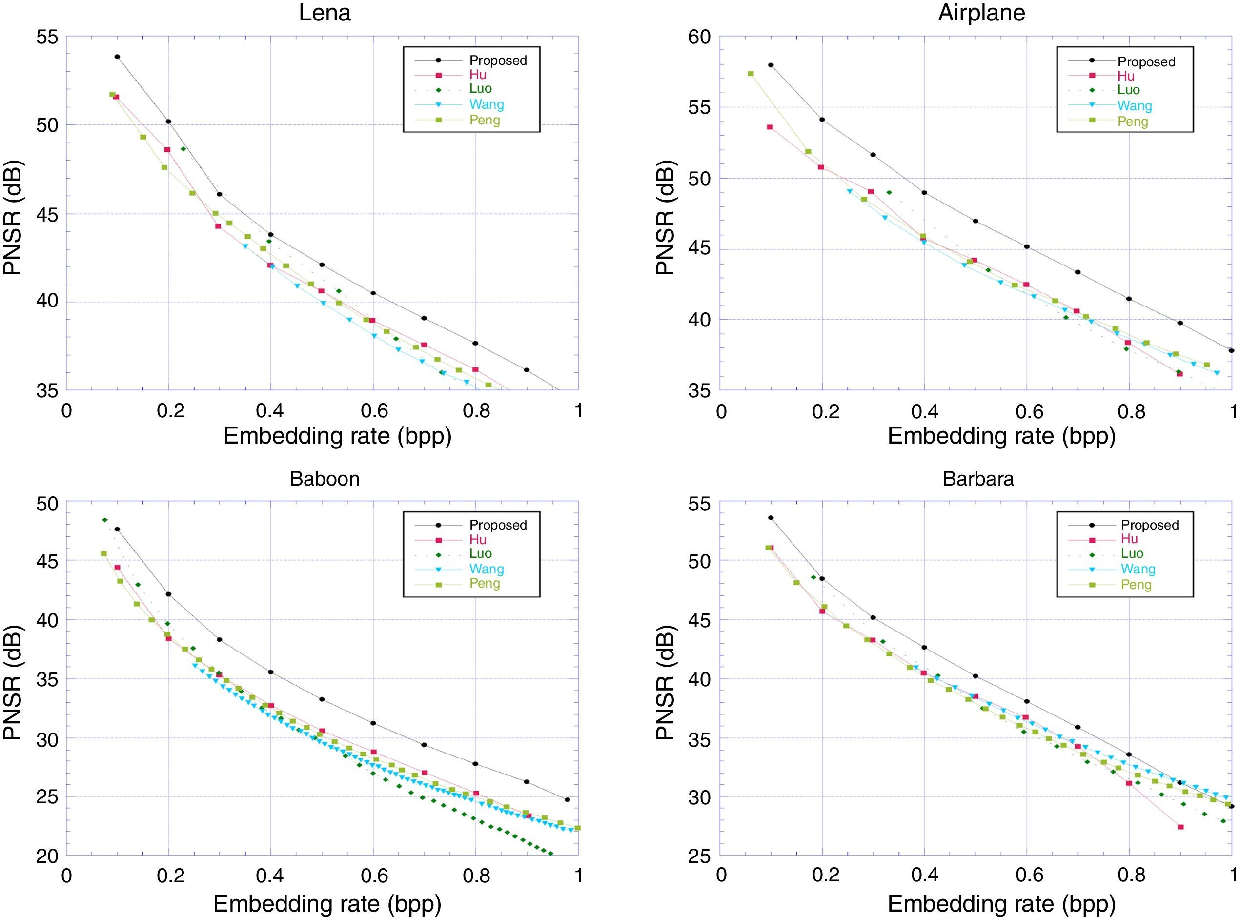
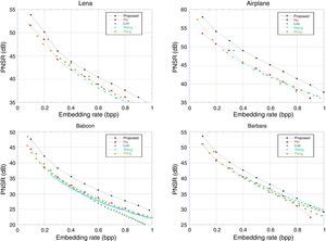
The method is assessed by comparing with Hu et al. (2009), Luo et al. (2010), Wang, Li, Yang, and Guo (2010) and one of the recent works by Peng et al. (2012). Results are compiled over the standard grayscale images of Lena, Airplane, Barbara and Baboon of size 512 × 512. The images are shown in the Fig. 5. The imperceptibility results are given in Fig. 6. The superior performance of the proposed method can be observed over all the test images. Improvement in results is primarily due to the use of high performance D-Mean predictor in the prediction mechanism. Maximum payload that can be embedded in a single pass of the proposed method is at most 1 bpp. Hence, for large payload size, the method should be applied iteratively.

Fig. 5.

512 × 512 sized, grayscale test images. From left to right are, Lena, Airplane, Baboon and Barbara.

Fig. 6.

Performance comparison between proposed method and that of Hu et al. (2009), Luo et al. (2010), Wang, Li, Yang, and Guo (2010) and Peng et al. (2012) over standard images.

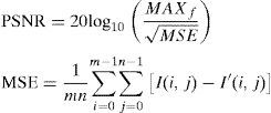
Selection of appropriate value for Edge sensitivity threshold T_S, is important for predictor performance. In this work the T_S is empirically determined and a value of 5 is used. It may be observed that the EC threshold controls the dual behavior of the predictor. For smaller values of T_S the predictor will act like median of four pixels, while large value of the threshold will make the predictor similar to mean predictor. An image, I after watermark embedding phase is noted as, I′. Imperceptibility test of the methods is carried out based on PSNR for a specific bpp (bits per pixel). Higher PSNR is always desired. It can be computed using Eq. (19). Comparison based on PSNR measure of watermarking methods is provided in Fig. 6. Imperceptibility test for a specific bpp of 0.5 is provided in Table 4. An average of 2.14 (dB) improvement in PSNR can be observed in comparison to Peng et al. (2012):

MAX_f for an 8 bit grayscale image is 255.

Table 4.

Comparison of PSNR (in dB) at an embedding rate of 0.5 bpp.

	Proposed	Hu (2009)	Luo (2010)	Wang (2010)	Peng (2012)
Lena	42.13	40.65	41.05	39.9	40.6
Airplane	46.98	44.26	44.21	43.07	43.52
Barbara	40.23	38.51	37.93	38.44	37.91
Baboon	33.26	30.63	29.46	29.48	30.29
Average	40.65	38.51	38.16	37.72	38.08

6

Conclusion

In this paper, a novel D-Mean predictor is proposed for PEE based reversible watermarking methods. D-Mean is state-of-art predictor which outperformed MED and GAP. D-Mean better models the presence/absence of an edge and uses 4 pixels around a pixel context which led to reduction in prediction-error. The method is simple and can be easily incorporated in the existing systems. Due to reduced overflow situation, location map shrinks to smaller sizes. The advantage of using D-Mean proved useful and results are improved for PEE based method. Future researchers may like to devise a scheme to auto-tune the parameters used in the D-Mean predictor and watermark embedding routine.

Conflict of interest

The authors have no conflicts of interest to declare.

Acknowledgements

First author would like to thank Higher Education Commission, Pakistan for funding a PhD fellowship under indigenous scheme through the grant no. 074-0941-PS4-070.