Effective planning of a transportation network influences tactical and operational activities and has a great impact on business. Planning typically considers multiple aspects such as variable transportation costs, various levels of customer service offered, security of goods, and traveling time. These aspects often vary with time. Although the minimum cost flow problem is a widely seen approach to configure a transportation network, there is no much work considering variations on arcs; even more, the problem with varying nodes has hardly been addressed. In this work is developed a mathematical model for the multi-objective minimum cost flow problem, applied in networks with varying attributes on arcs. The model finds the set of non-dominated solutions for a multi-objective stochastic network having variations in attributes of its arcs and nodes, such as cost or transportation time. A modified version of the two-stage method was used to address the stochastic nature of the problem combined with the epsilon-constraint method, which is used for building the set of non-dominated solutions.
This paper presents the main features of the model, the theoretical bases and a computational implementation. Experiments were applied in a transport network for the exportation market of ornamental flowers as perishable goods from Mexico to the United States, which considered variations in border crossing times.
Una planeación eficaz de una red de transporte tiene un gran impacto en las empresas, al considerar múltiples aspectos como costos de transporte, seguridad de las mercancías, tiempo de viaje y demás niveles de servicio ofrecidos. Atributos que frecuentemente varian con el tiempo. Aunque el problema de flujo a costo minimo (MCF) ha sido ampliamente visto para configurar redes de transporte, no hay muchos trabajos que consideren variaciones en los arcos. En este trabajo se desarrolla un modelo matemático para el problema MCF multi-objetivo, aplicado en redes con atributos variantes en los arcos. El modelo encuentra la Frontera Pareto para una red estocástica con variaciones en los atributos de costo o tiempo de transporte. Para enfrentar la naturaleza estocástica del problema se utiliza Descomposición de Benders para el problema estocástico de dos etapas, posteriormente se conjunta con el método ¿-restricción, que es utilizado para la construcción del conjunto de soluciones no dominadas.
Este articulo presenta las principales características del modelo, las bases teóricas y una implementación computacional. Los experimentos fueron aplicados en una red de transporte para el mercado de exportación de flores ornamentales como productos perecederos desde México a Estados Unidos, considerando las variaciones en los tiempos de cruce de fronteras.
According to the Strategic Technology Observatory of the Tecnologico de Monterrey in Mexico [1], the State of Mexico has shown growth rates below the national average in recent years, despite this, the agricultural sector showed an average annual growth of 3.1% to 2011. In the agricultural sector, an opportunity is in the planting of ornamental flowers. Planting of chrysanthemum, rose and carnation in the south and east of the state represents the 19.33% of the total value of production using only 0.38% of the sown area.
While is globally recognized that Mexican flower quality is excellent, the main challenge for all actors involved in the floriculture industry is to take them to the homes, and promote consumption as a frequent habit.
Proximity of Mexico to the United States, the main buyer of flowers outside Mexico, gives the country a competitive advantage in this market relative to its competitors like Colombia and Ecuador, allowing better travel times for trucking transport and the resulting cost savings compared to air mode, a condition that can only be used by Mexican producers [2, 3].
Despite its contribution to the transport network design, the Minimum Cost flow problem (MCF) is far from adapting to the needs of transport that companies may have, which routes need to select suppliers from different objectives, not only from choosing the lowest cost or the shortest time separately. In various applications in real problems of route selection are considered other targets, so that the identification of a unique solution that is better to others with respect to all objectives is often impossible, rather than a single solution is sought a set of Pareto optimal solutions. This problem is known as Multi-Objective Minimum Cost Flow (MMCF).
In MMCF, [4] found that the majority of the approaches are of theoretical interest. It was also found that although for continuous MMCF, approximate algorithms for finding a representative set of all efficient flows generate good quality results, the appropriate approach to the entire case (MMCIF) has hardly been addressed by current literature in [5, 6, 7, 8, 9].
Unlike deterministic models, this paper considers variations in transportation time attribute on arcs corresponding to the crossing borders. In this arcs were considered three possible states for crossing times (low, medium, high) with its respective probability of occurrence. The resulting problem grows exponentially according to the number of variant arcs with respect to deterministic model.
The kind of problem to be solved relates to the determination of an efficient curve that provides various appropriate routes optimizing interest objectives for the distribution of perishable goods in constrained networks, where the time dependence and the stochastic nature of attributes on arcs and capabilities are explicitly mentioned. The resulting model will serve to solve the Multi-objective Minimum Cost Flow problem for stochastic networks (SMMCF).
In [10] was proposed to test this model the International Trade U.S. – Mexico for perishable products, in a particular problem of exportation from a Mexican region to destinations in the U.S., where there are variations in arc attributes such as travel time, mainly due to delays in nodes. This is a problem of multi-objective minimum cost flow, with time variations in arcs and in certain nodes, which may result from the congestion, it is applied to the case of flower export market, having its origin in the State of Mexico and Puebla, and identifying different possible destinations in the U.S. It's about finding the flows of merchandises minimizing costs in both, monetary and time terms.
In Section 2, concerning the description of the problem, will deal with the nature of the problem to solve, which by its nature is considered a minimum cost flow problem with multiple objectives and stochastic variations in their arcs. To deal with variations in arcs, is proposed the use of the two-stage method, which will be solved by Benders decomposition, these techniques are described in Section 3. Later, in Section 4 is developed a model to deal with the stochastic multi-objective minimum cost flow problem. Finally, Section 5 discusses the work done, explaining the application instance and the characteristics of the developed program for its solution, presented difficulties and solutions found.
2Multi-objective minimum cost flow problemAccording to [11] the group of problems currently known as transport problems was first studied in [12]. In turn, another seminal work [13] described the standard form of transport problem. Here was proposed a method for finding the fixed points in this border, called vertices, to generate better solutions iteratively expressing the objective function in terms of zero-valued variables.
Much of the development known as minimum cost flow problem (MCF) and network-based methods are attributed to [14]. MCF has been studied by many authors as in [15, 16, and 17].
A multi-objective linear problem (MOLP – multi objective linear problem) is given by
where C=(c1, …, cp) with rows C1, …, CP denotes a linear matrix p×mIn MOLP conflicting objective functions are assumed, i.e., excluding the existence of an ideal solution x∈X that minimizes all objectives p simultaneously. According with [18, 19 and 8] a solution y′∈Y is not dominated if no other solution y∈Y such that y≤y′ and y≠y′.
There is a variety of available methods to solve multi-objective problems; many of them involve converting this in one or a series of single-objective problems [20, 21, 22, 23 and 24].
¿-constraint method is proposed to solve the MMCF problem because, within scaling methods is the best suited to mixed integer programming problems and guarantees to obtain all Pareto border points (as a trade-off with run time).
2.1¿-constraint method¿-constraint method was proposed in [25, 26], where this method is based on an escalation where one of the objective functions is bounded by additional restrictions
Where ¿k=(¿1, ¿2, ¿k-1, ¿k+1, ¿p)T ∈ Rp-1 and k∈{1, …,p}. The feasible set of the problem is given as:Theorem 1. x* is an efficient solution of a biobjective problem if and only if ∃¿2 such that x solves P1(¿2) or ∃¿1 such that x* solves P2(¿1).
Theorems 1 has been demonstrated for general multi-objective problems in [25]. This means that efficient solutions can always be found by ¿-constraint method.
Theorem 1 indicates that, for every efficient solution x*, can be found a ¿j such that x* can solve P1(¿j) or P2(¿j), with this, the complete Pareto frontier can be found by solving ¿-constraint problems.
According to [27], calculating the range of the objective functions on the efficient set is not a trivial task, while the best value is easily accessible as the individual optimum, the worst value in the efficient set (nadir value) is not. The most common approach is to calculate a set of these ranges from a trade-off table (the table with the results of individual optimization of the objective functions p), where nadir value is usually approximated with the minimum column.
In [27] was proposed a transformation of equality constraints on the objective function by explicitly incorporating the appropriate slack. At the same time, the sum of these slack variables is used as secondary terms (lower priority) in the objective function to force to only produce efficient solutions. The new problem becomes:
where ¿ is a small number (usually between 10−3 and 10−6)In [27] was also performed and demonstrated the following proposition: the above formulation of the ¿-constraint method produces only efficient solutions (avoiding the generation of weakly efficient solutions).
¿-constraint method works predefining a virtual grid in the objective space and solving different single objective problems restricted in each grid cell. All of Pareto optimal solutions can be found only if grid is fine enough that at most one Pareto optimal solution is found in every cell. For a general problem, the choice of the grid size parameter is therefore very difficult besides, but influences also the execution time of the algorithm.
The steps to follow in the ¿-constraint method are:Algorithm 1¿-constraint method Set k1 (k) as the first target to consider, km1(k) to other objectives. Set kk(k) to the objective function as a constraint in a single expression, this is done with objective functions different to k1(k). Optimize the first objective and the others are set as constraints. Generate the trade-off table with lexicographic optimization. Release the fixed values of the objective functions for a new iteration. Define different grid intervals for different targets. Walk the grid points and take shortcuts, if the model becomes feasible. Keep going on the net. Get unique solutions from the point file.
To solve problems with variations in the arcs is proposed the two-stage method [28].
According to [29] a linear stochastic two-stage program with stochastic fixed resource is a two-stage program with the following form:
where Q(x, ¿) is the optimum value of the second stage problem.The second stage problem depends on the data ¿ (¿)≡(q (¿), h (¿), T (¿)), which elements can be random, while the matrix W is known beforehand. Matrices T(¿) and W are called matrices of technology and resource, respectively.
The expectation IE [Q (x, ¿)] is taken with respect to the random vector ¿=¿(¿) whose probability distribution is assumed to be known. The above formulation was originated in [30].
Whereas the optimal solution y* = y*(¿) of the second stage of (5) may depend on the random data ¿ = ¿ (¿), and hence is random, it has
If the random data have a discrete distribution with a finite number K of possible realizations ¿k=(qk, hk, Tk), k=1, …, K, (scenarios) with their corresponding probabilities p(k). Then
whereTherefore, the problem of two stages can be formulated as a big linear problem: min cT × +nkpkqTk yk
Linear problem (8) has a concrete block structure that makes it susceptible to various decomposition methods.
The above numerical approach works reasonably well if the number of scenarios is not too large. However, if the random vector ¿ has m components independently distributed with only 3 possible realizations. Then the total number of different scenarios is K=3m. That is, the number of scenarios grows exponentially with the number m of random variables. In that case, even for a moderate number of random variables, for example m = 100, the number of scenarios becomes so large that even modern computers cannot deal with the required calculations. To deal with exponential growth in the number of scenarios is proposed using Benders decomposition method.
3.1Benders DecompositionA major concern regarding the building and solving of optimization problems is that the computational effort required to solve such problems grow significantly with the number of variables and constraints. The traditional approach, which involves making all decisions simultaneously by solving a monolithic optimization problem quickly, becomes intractable because of the increase in the number of variables and constraints. The multistage algorithms for optimization, such as Benders decomposition [31], have been developed as an alternative approach to palliate this problem.
Unlike the traditional approach, these algorithms split the decision making process in several stages. In Benders decomposition, a main problem is solved in its first stage for a subset of variables, while values of the remaining variables are determined by a subproblem of the second stage, given the values of variables of the first stage. If the subproblem determines that the proposed decisions in the first stage are not feasible, it generates one or more constraints and added to the main problem, which is then solved. Thus, a series of smaller problems are solved instead of one big problem, which can be justified by the increase in computational resource requirements associated with the solution of larger problems.
The MIP problem can be set as [32]:
If y is attached to a feasible integer configuration, the resulting model to solve is:
Full minimization problem thus can be written as:
Then, the dual internal LP problem is:
Under Benders decomposition two distinct problems are solved. A major problem which has the form:
and subproblems with the form:The dual subproblem is a linear programming problem, and the main problem is a pure IP problem (no continuous variables). Benders Decomposition for MIP is of particular interest when the Benders subproblems and the relaxed master problem are easy to solve, while the original problem is not.
4ModelsAs mentioned, in this paper is proposed to add the component of variation in attributes of certain nodes at the multi-objective minimum cost flow problem. Since it has been seen that in current state of art there are few studies that take into account changes in attributes on arcs and this is compounded if there are problems with variations of attributes in nodes.
The proposed model to work with multi-objective minimum cost flow problems adapted to deal with variations in the attributes of the arcs and nodes, was based on the classic MMCF models. With this, the two-stage model applied to a MCF problem would be as follows:
i Set of node indices of arc source, i∈V
j Set node indices of arc destination, j∈V
cijp Relative cost to use the arc from i to j in accordance with criterion p, p=1,2,…,r, (i,j)∈A
xij Flow from i to j nodes, i,j∈V
bi Capacity/demand of node i, i∈V
E[cijp] Expected value of relative cost to use the arc from i to j in accordance with the criterion p, p=1,2,…,r, (i,j)∈A
Pq Probability of scenario q, q=1,2,…,Q
Cqijp Relative cost to use the arc from i to j in accordance with the criterion p in a scenario q, p=1,2,…,r, (i,j)∈ A, q=1,…,Q
P[cijp] Probability of cost value for using arc (i,j) for criterion p on scenario q, p=1,2,…,r, (i,j)∈A, q=1,…,Q
xqij Cargo flow from I to j for scenario q, (i,j)∈A, q=1,…,Q
s.t.For all i=1,…,g (second stage)
i=1,…k in deterministic arcs
i=k+1,…m in stochastic arcs
q=1,…,Q scenarios
The first set of terms in (15) represents the expected values already known and which fall in the first stage of the problem. This has the classic form of the multiobjective minimum cost flow problem as in (1), where the objective is to minimize the cost of for the p attributes of sending the merchandises from a set of origins to a set of destinations. This set includes the objectives for which all values are deterministic and the known values of stochastic objectives. The flow conservation constraints on nodes connected by arcs with known values are defined in first group of terms of (16).
On the other hand, the second set of terms in (15) represents the data of which there is uncertainty in the values it takes, but where are known both the possible values that could be taken as the probability that these values are presented. Formulation is similar to first group of terms, but considering the probability of each scenario. Second group of terms in (16) refers to the flow conservation in those nodes connected by arcs with non-deterministic values, where probability of scenarios affects the expected flow.
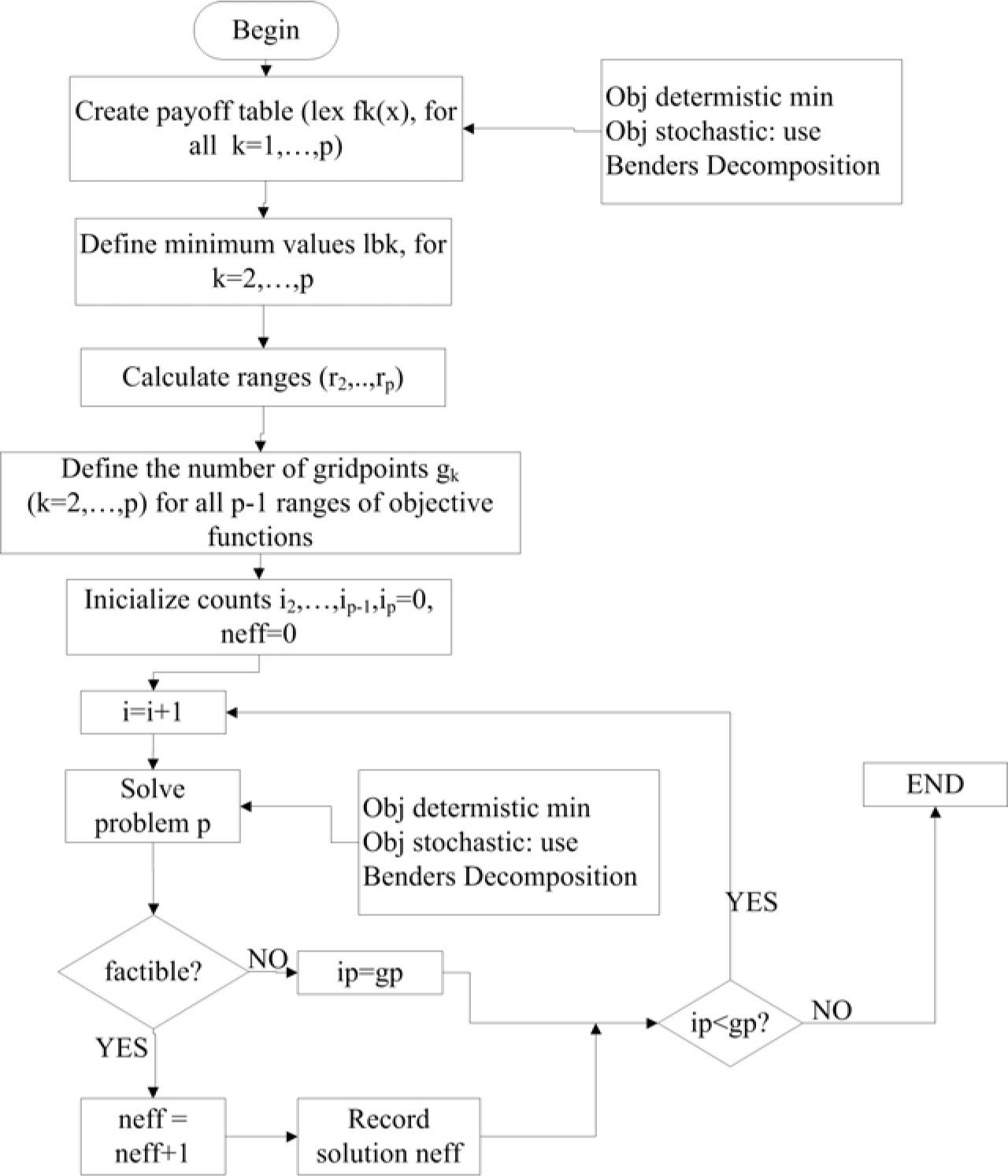
Selected methodology includes the two-stage method to develop scenarios that could arise depending on the state of time on the variant arcs and their respective probabilities. Once scenarios are generated, the method applies ¿-constraint to solve the MMCF problem, using Benders decomposition in stochastic arcs as in Figure 1.
It is noteworthy that objectives which all arcs are deterministic are optimized to generate the tradeoff table as described in Section 2. To generate the trade-off table should minimize the first goal and the resulting value is used as a restriction to minimize the second objective, this procedure is repeated but the second objective is minimized at first and it is used as a constraint in minimizing the first objective.
To estimate each grid value on all objectives with stochastic arcs, Benders decomposition is applied in step 9 of Algorithm 1 when k1(k) corresponds to objectives with variations in arcs.
5ApplicationThe problem is exemplified by a dealer of flowers located in Tenango, State of Mexico and Tecamachalco, Puebla. Its main client is in Chicago, Illinois, so that the transport of flowers is of great importance.
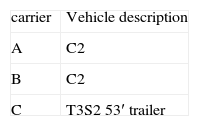
The goal is to bring flowers on a weekly basis, so is being looking to choose the best route. To illustrate the process were considered three transport companies on the Mexican side, which can use two different types of transport units:
Each path is characterized by the transport provider company, the type of vehicle used by the operator, the transshipment center (or if is a direct ride to the border) and the border crossing point used. This instance considers only one transport service provider in the United States.
In turn, can be used four transfer centers which are located in Queretaro, San Luis Potosi, Aguascalientes and Zacatecas, and four border crossings: Colombia in Nuevo Leon, and Nuevo Laredo, Reynosa and Matamoros in Tamaulipas.
At each border crossing there is the option of hiring a specialized carrier to cross the merchandise from one side to another of the border (transfer), or do so directly by a Mexican or American vehicle having the proper permits to cross the border.
Within bilateral initiatives developed to ensure safe and efficient flow of goods is that of FAST/Express lanes, applicable to Mexican companies that have been certified in the Customs-Trade Partnership Against Terrorism program (C-TPAT). This is aimed at reducing waiting times at the common border creating a more streamlined flow of vehicles in both directions.
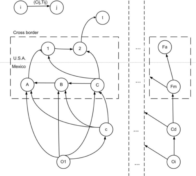
Figure 2 summarizes the activities carried out on the border between Mexico and the U.S. and displayed the characterization of a border crossing.
- •
Where the same border crossing (formed by the dotted box) consists of nodes A, B, C on the Mexican side and 1, 2 on American side.
- •
From an origin Oi vehicles can travel directly to the Mexican border or through a distribution center c.
- •
The arcs that reach nodes A and B represent two different C2 vehicles while C comes by T3S2.
- •
Arc A-1 represents the border crossing by means of “transfer” service, while in C-1 is performed by T3S2 and C-2 by T3S2 using the “Fast” lane.
Transport attributes considered in the study are the following:
Cost. This refers to the amount of resources used to carry out the transport given its efficiency, as the generation of wealth and income by transporting goods.
In the case of perishable goods, since they have a limited lifetime, is establishing a minimum lifetime shelf. To be able to complying with the shelf life time, transport time should not exceed a value Tan, as each unit of time is exceeded in transport represent deterioration in the condition of the goods. The deterioration of the goods can be considered as an increase in the total cost of transport, so that the total transportation cost in (17) for the objective of cost would be represented as follows:
Where:
Cij is the price of transport service incurred when crossing an arc in the network.
Dij is the cost due to deterioration of goods due to excessive transportation time.
Time. One of the objectives to be considered is to minimize the total transportation time from the beginning to the final destinations. For this, the time data for arcs are considered deterministic, except for the arcs corresponding to border crossings, in which time will have three states that may occur (low, medium, high) and the likelihood that they will arise.
For the travel time attribute in (16) shows the modification to the time objective:
Where:
E[tij]Xij Is the expected value (considered as deterministic) of time to cross an arc within the network
[tqij]Xqij Is the time to cross an arc in the network given the scenario q
P(q) Is the probability that arc (i, j) is in the state q
Under these conditions was formed a network of 29 nodes and 158 arcs, of which 12 arcs depicts activities at border-crossings and can take three states of time: low, medium, high. Cost data are taken as deterministic, while time is considered as stochastic since it was considered variability in time to cross some arcs.
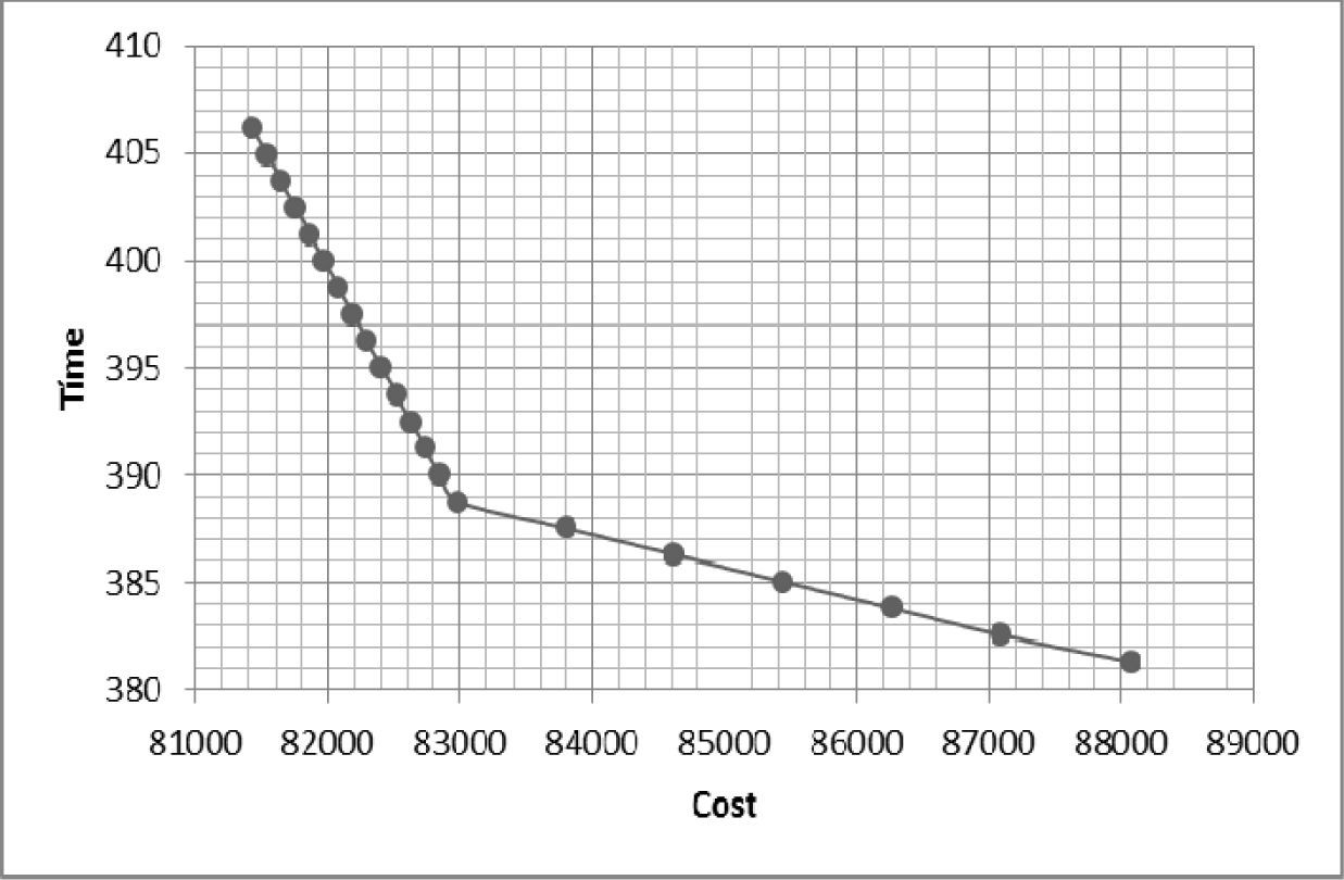
In implementing Benders decomposition, cost attribute and constraints corresponding to equilibrium at nodes connected by arcs with deterministic times, are reported in the first stage, while those elements that represent uncertainty as the time attribute and equilibrium constraints on nodes where involved arcs have varying times, are reported in the second stage. This will generate time and cost options that subsequently feed the ¿-constraint method. Figure 3 shows the Pareto frontier obtained with the results of non-dominated routes for the exporting perishable products.
Tests were conducted to the same network where was considered that all arcs have deterministic times, for which the expected values E [tij] were used. While in these arcs the maximum times were around 2.5 to 10 times the mean time, the results obtained for routes on the Pareto frontier, times showed values around 0.14% higher than the deterministic equivalent problem. The problem in stochastic version has the advantage that it provides the flexibility to consider variations in arcs, while the resulting paths are slightly higher in transport time.
In the attribute of time, given the ranges in the stochastic model as in the deterministic model, which intersect at most of them, from T test to compare means, does not give elements to reject H0 given the level of significance shown. Furthermore, a Levene analysis were performed for equal variances, the result is that the time for variances obtained by stochastic and deterministic models are different with a significance level of 0.128, therefore, there are evidence to reject the null hypothesis. Table 1 shows the results of tests for equality of mean and variance. This comparison between means and variances shows that Pareto frontiers generated by stochastic models have a different distribution to those generated by deterministic models.
Comparison of time in case of application for stochastic vs. deterministic model.
| levene test for equality of variances | levene test for equality of means | ||||
|---|---|---|---|---|---|
| F | Sig. | t | gl | ||
| assuming equal variances | 2,531 | 0,128 | 6,805 | 19 | |
| without assuming equal variances | 7,584 | 18,957 | |||
| T test for equality of means | |||||
| Sig. (bilateral) | diffe rence of means | standard error of the difference | confidence interval for the difference 95% | ||
| Low | Up | ||||
| assuming equal variances | 0,000 | 1304,769 | 191,741 | 903,451 | 1706,087 |
| without assuming equal variances | 0,000 | 1304,769 | 172,052 | 944,605 | 1664,933 |
It has been shown that the ¿-constraint method can be efficiently used to find the exact Pareto multiobjective problem. Benders decomposition is useful to solve problems with variations in arcs.
In SMMCF instances, when comparing the ranges on the Pareto Fronts, results show that this type of model tend to generate slightly higher values of time and cost in stochastic version than in deterministic version in which were used expected values. This same behavior should occur in different networks, although the degree of variation between stochastic and deterministic curves depends on the difference between the values of time state in arcs (low, medium and high).
The approach developed for SMMCF is generalizable to problems with the following characteristics:
- •
Perishable products, in which the time of transport has a significant impact.
- •
Export products where congestion at border crossings produces variations on service times, which can be discretized.
- •
Markets with multiple origins and destinations.
- •
Selecting routes based on suppliers with different capacities, costs and time services, depending on the characteristics of its fleet
The proposed approach works with the probability of occurrence of each scenario, so that gives the set of routes with shortest probable time, rather than working with expected times.


