Se desarrolla un marco para tasar las opciones energéticas asiáticas sometiendo el valor del activo subyacente a un método de fracciones discontinuas. La ecuación en derivadas parciales (EDP) en el entorno fraccional con salto se construye para una opción dada utilizando la fórmula general de Itô y una estrategia dinámica de autofinanciación. Con la condición límite, resolviendo la EDP se deriva una fórmula analítica para la opción con una media geométrica que empieza en cualquier momento antes de la madurez, y la opción con media aritmética se evalúa con simulación de Monte Carlo utilizando variables de control apoyadas en la citada solución analítica. Hay abrumadora evidencia numérica de que la técnica propuesta es eficiente en tiempo de cálculo y mejora espectacularmente la precisión del precio simulado. Es más, este estudio abrirá un nuevo camino que seguir en los contratos de opción de compra basados en bienes tan poco negociables como el petróleo, las divisas o los tipos de interés.
A framework for pricing Asian power options is developed when the underlying asset follows a jump-fraction process. The partial differential equation (PDE) in the fractional environment with jump is constructed for such option using general Itô's lemma and self-financing dynamic strategy. With the boundary condition, an analytic formula for the option with geometric average starting at any time before maturity is derived by solving the PDE, and the option with arithmetic average is evaluated in Monte Carlo simulation using control variate technique with the help of the above analytic solution. Overwhelming numerical evidence indicates that the technique proposed is computationally efficient and dramatically improves the accuracy of the simulated price. Moreover, this study will pave a novel way to copy with the option contracts based on thinly-traded assets like oil, or currencies or interest rates.
1. Introduction
All kinds of exotic options arise one after another in the environment of volatile financial market. Asian power options are successful. They have become widely used in the fields of stock, commodity, energy and foreign exchange. Kemna and Vorst (1990) proposed an analytic expression for Asian options with geometric average using the partial differential equation (PDE) approach, on this basis, geometric average as control variable employed in the Monte Carlo simulation method (Boyle, 1977) was used to obtain satisfactory result for pricing Asian options with arithmetic average. Chen and Lyuu (2007) came up with a close-form solution for arithmetic Asian option using the approximation of arithmetic average through geometric average appeared. The approximate approach works as well as the Monte Carlo simulation approach but accuracy remains problematic for high volatility and/or long maturity cases. In addition, lattice binomial method (Hull & White, 1993; Neave & Turnbull, 1993) has been proposed to handle Asian options. But it has a dramatic computational cost because a large number of possible realizations of the payoff must be considered. Among the above most common methods to price Asian options, Monte Carlo method is rather simple to implement and can provide standard errors for the estimates to measure quality, and it further achieves a satisfactory level of accuracy with the enhancement of control variate technique for more complex arithmetic average option (see Boyle et al, 1997). At the same time, the analytic solution of the Asian option with geometric averaging is indispensable in the control variate technique and PDE approach (Alziary et al., 1997; Zhang, 2001) provides an accurate result for geometric average option without computationally expensive when the PDE to be solved has three or four independent variables. As far as power option is concerned, Blenman and Clark (2005) explicitly solve for the price of the power option to exchange one asset for another under the equivalent martingale measure in which they specified that the price of power call is equal to the price of the power exchange option when the power of another asset is zero.
Most of the academic researches on such exotic options assume that the underlying asset evolves as a continuous diffusion process. This implies that logarithmic returns of the asset are normal random variables. However, empirical evidences in Jorion (1988), Bates (1996), Pan (2002), Chernov et al. (2003), and Eraker (2004) indicate the presence of discontinuous jump in asset price when significant new information or catastrophic events arise. The jump-diffusion process is widely used to model jumps of the price movement and was introduced to option evaluation by Merton (1976) and Gukhal (2004). In recent years, many empirical studies on capital market also show that the logarithmic returns on financial assets are not normally distributed but the distribution with excess kurtosis and fat tail. Moreover, price series on financial assets are not stochastic motion but long-range dependence. Peters (1989) found the fractal structure and non recurrent phenomenon in both stock and exchange rate market and proposed the hypothesis of fractional market. Fractional Brownian motion, as a family of Gaussian processes, can give a satisfactory description of the price dynamics of the underlying asset because it has two important properties of self-similarity and long-range dependence. Considering fractional Brownian motion is neither a Markov process nor a semi martingale, Duncan et al. (2000) built up the fractional-Itô-integral to analyze it. Furthermore, Hu (2003) proofed that the option market under the fractional Brownian motion is perfect without arbitrage opportunity using the Wick integration and gave European option pricing formula at arbitrary time. Indeed, some authors have used the fractional Brownian motion to capture the behavior of underlying asset and to obtain fractional Black-Scholes formulae for pricing options including Necula (2002), Bayraktar et al. (2004) and Meng and Wang (2010).
To better describe the evolution of asset price, the combination of Poisson jumps and fractional Wiener process is introduced in this paper. The jump fractional process is consistent with an efficient market where major information arrives infrequently and randomly. In addition, this process is capable of capturing the empirically observed distributions of asset price changes that are leptokurtic, skewed, long memory and have fatter tails than comparable normal distributions, and provides a good explanation for volatility smile effect of log normally based Black-Scholes model. That is, the implied volatility varies with moneyness and maturity.
The problem of pricing option when the underlying asset value is driven by a jump fractional process was solved by Xiao et al. (2010) who derived a pricing model for currency option value. Things are more complicated in the case of exotic path-dependent option such as Asian power options developed in this paper whose payoff depends on the geometric or arithmetic average of the underlying asset raised to power. Such option represents a simultaneous generalization of Asian options as well as power option both of which play an important role in the risk management and incentive contract (see Zhang, 1997, Tompkins, 1999). The average feature embedded in power option makes Asian power option less subject to price manipulation thus hedging nonlinear risk arising in option positions from changing level of implied volatility and smoothing randomness inherent in the stock price so that the managers can be evaluated more fundamentally in the incentive contract for indexed executive option compensation. Despite many literatures on Asian option, there is litter work on Asian power option.
The objective of this paper is to study the pricing of Asian power options with geometric and arithmetic. Meanwhile we capture the behavior of the underlying asset using the jump-fraction process and follow the control variate technique whose chief advantage is its high accuracy and efficiency. The outline of the rest of the paper is as follows: The next section derives the analytical formula for the Asian power options with geometric average using PDE approach after giving the assumption of pricing environment. Section III demonstrates how the analytical solution as control variable is implemented in the Monte Carlo simulation to obtain an accurately simulated price of the Asian power option with arithmetic average. Conclusions are presented in the final section.
2. The valuation model
Consider a complex and f lexible financial economy where information arrives both continuously and discontinuously. This is modeled as a continuous component with the features of "asymmetric leptokurtic" and "long memory" and as a discontinuous component with abnormal fluctuation in the price process. Assume that the asset pay dividends, the price process can hence be specified as a superposition of these two components and can be represented as;
where μt and qt are time-dependent parameter respectively denoting expected yield rate and dividend rate. s is volatility; Bt H
is a fractional Brownian motion with Hurst parameter H∈(0, 1) which is Centered Gaussian process with mean zero and covariance
; Qt is a Poisson process with intensity λ, dependent of Bt H, Nt is Poisson compensation process and equals Qt-λt.
Theorem 1 Set Wt=BtH + Nt, fl(t,ϕ) ∈ C1,2 (R+ × R → R) and f (t,Wt),
belonging to L2(P), then
Proof: See Appendix A
Theorem 2: The solution of the stochastic differential equation (1) equals
the theorem can be proven from Theorem 1.
Theorem 3: Consider an Asian power option with contingent claim process V(St, It) ∈ C1,2 (R+ × R → R) , written on the risk asset following (1), the partial differential equation in the jump fractional environment is
Proof: Since Asian power option is path-dependent option whose price is related to path factor besides time and the underlying asset. We introduce a new variable
Let the option price at t (0 ≤ t ≤ T) be V (St It, t) the option value is path-dependent on It but it is fundamentally driven by the original underlying assets in (1), whose dynamics is derived by applying Lemma 1 and Lemma 2.
We replicate the option by constructing the hedging asset portfolio composed of the risk asset St. And bond Bt with riskless interest rate r θt0 andθt1 represents the position of risk asset and riskless asset held in the portfolio, then the wealth process V =θt0Bt +θt1St. Using self-financing dynamic trading strategy:
Consequently we can obtain the result of Theorem 3.
3. An analytic formula for Asian Power Option with geometric average
Because the geometric average of a so assumed variable remains in the family of the Itô process, we price a European-style Asian power option on geometric average with maturity T and strike price K by solving the partial differential equation (4).
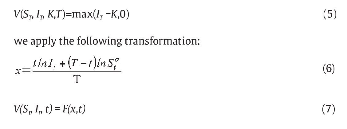
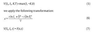
Given the boundary conditions of call option
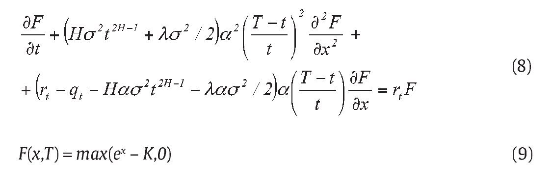
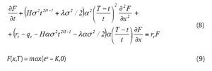
to equation (4) and (5) to yield
where equation (8) after an appropriate change of variables, becomes a classical heat equation (see, e. g., Daly & Logan, 1998). Further, we apply the following transformation
and
to equation (8) and (9) to obtain
The solution to equations (13) and (14), which has been verified by us using Green's function approach, takes the following form
where: N(-) is the cdf of a standard normal distribution.
Thus the solution to equations (4)-(5) can be written as
where the function U(y, z) is given by (15), with
By doing some algebra, the solution to our problem (4)-(5) can be further written in the following result:
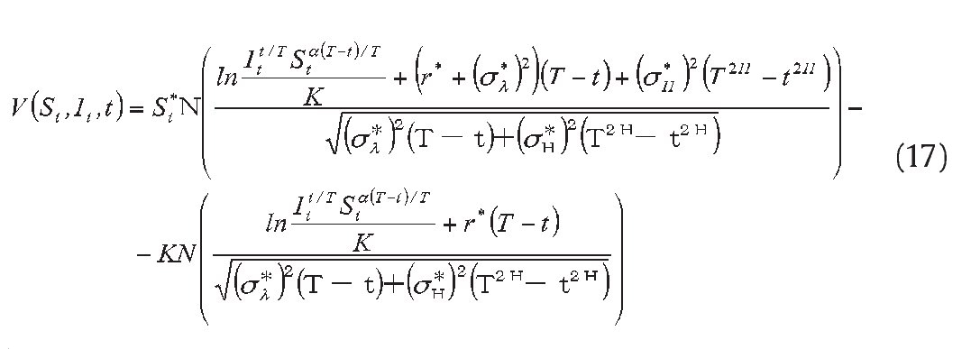
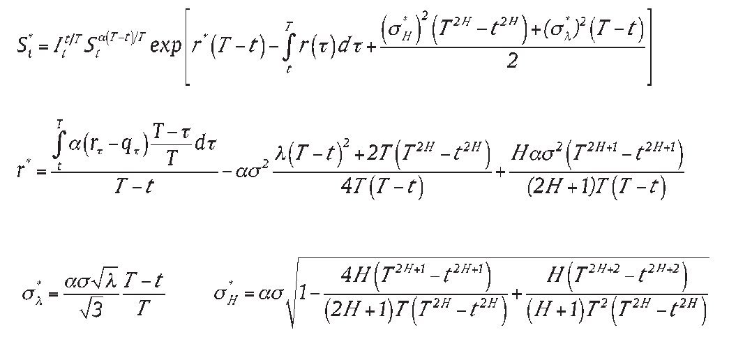
Proposition 1. The analytic pricing formula of a geometric Asian power call option with maturity T and strike K , path factor It , powerα, written on an asset following Eq. (1) is given from the solution to equation (4)-(5), i.e.
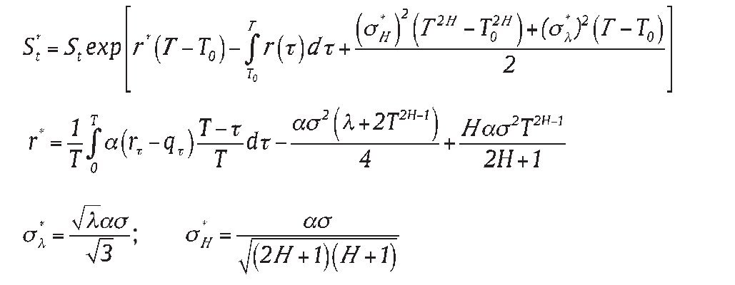
where
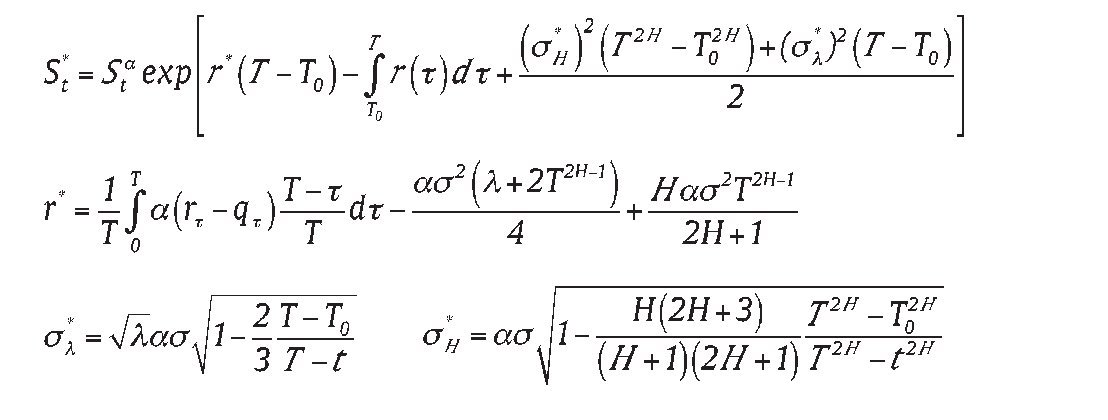
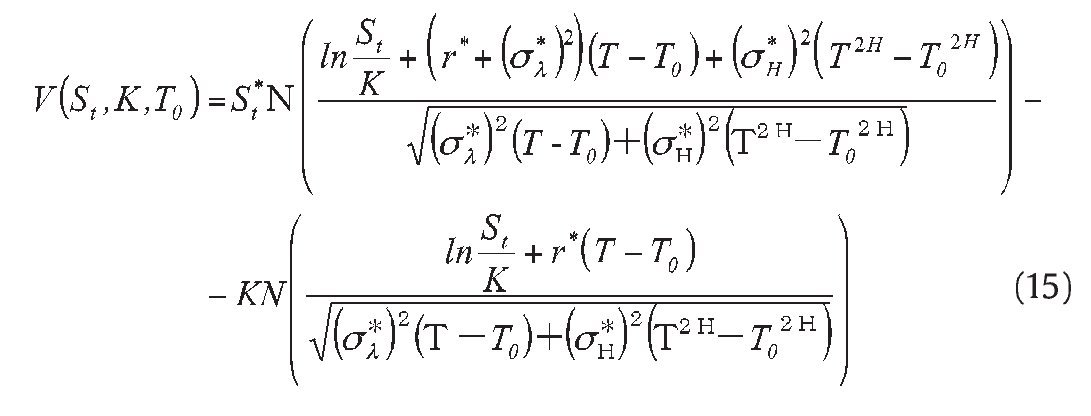
The above result can be extended to a forward-start-averaging Asian power option on geometric average price, we use time notations as follows: 0 = start of the option; t = option valuation date; T0 = start of the averaging; and T = maturity of the option or the end of the averaging. We assume 0 ≤ t ≤ T0 < T, with the forward-start-averaging taken over [T0, T]. The approach is to determine option price at T0 and evaluate it discounted expectations at t by integration, the final result is stated below (see Appendix B for the derivation):
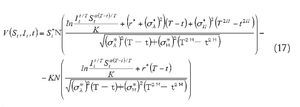
Corollary 1: The analytic pricing formula for the forward-start-averaging call option for geometric Asian power starting at T0, and expiring at T, with strike price K, power α, written on an asset following Eq. (1), is
where
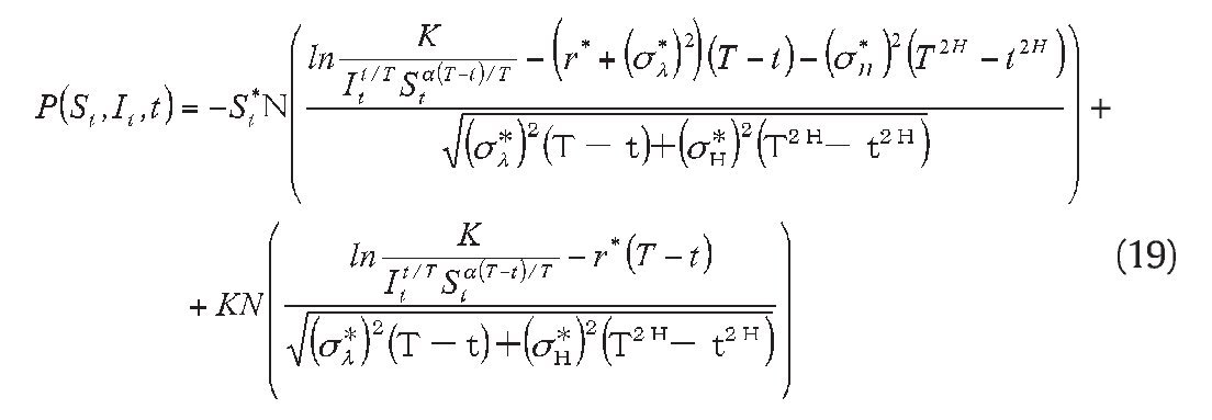
The put case can be derived in the same way as proposition 1. On the basis of boundary conditions P(ST, IT, K,T)=max(K - IT,0), we solve equation (4) and obtain the price of Asian power put option P(St, It, t).
Proposition 2. Geometric Asian power put option with maturity T and strike K, path factor It, power α, written on an asset following Eq. (1) whose analytic solution is given by
where St*, It, r*, σl*, σH* are as defined as proposition 1.
Expression for the case of forward-start-averaging put option can also be derived in a similar manner. Thus, the price of such option is presented as follows:
Corollary 2: The analytic pricing formula for the forward-start-averaging put option for geometric Asian power starting at T0, and expiring at T, with strike price K, power a, written on an asset following Eq. (1), is
where St*, It, r*, σl*, σH* are as defined as Corollary 1.
It is straightforward to verify that familiar pricing formulas obtain as special cases of (17)-(19). For example, for H=0.5, α=1, (17)-(19) reduce to the familiar jump-diffusion formula for the price of geometric Asian call and put options with fixed strike price K. Moreover, when λ=0, parameter q and r is constant, (17) and (19) simplify to the standard Asian option with geometric average on assets driven by geometric Brownian motion which is consistent with the result from Kemna and Vorst (1990).
4. Simulated price of Asian power option with arithmetic average
The pricing of European path-dependent option can always be implemented using the simple and efficient Monte Carlo simulation. The approach becomes the last resort especially when there is no analytical formula available for the pricing of Asian power option with arithmetic average because the arithmetic average of so-called assets does not remain in the family of the Itô process. One important issue in implementing the simulation method is the accuracy of the calculated option price which is measured by sample variance, and the relationship between them is negative; that is, the accuracy of the option increases as the variance decreases. The number of simulation runs depends on the accuracy. In general, the accurate simulated price can be obtained only by large number of simulation runs without adjusting the sampling method. To reduce the variance and achieve high accuracy of the simulation results for arithmetic Asian power option within a feasible number of simulation runs, the implementation of a control variate technique in the Monte Carlo simulation approach is necessary.
The control variate must be the financial derivative with positive relationship of the simulated derivative and derived analytical solution. The geometric average can serve not only as a lower bound for the arithmetic average but also as a control variate in the simulation approach. Thus, the analytical formula in proposition 1 and proposition 2 with geometric average becomes indispensable in the simulation approach to pricing of the options with arithmetic average because the formula plays an integrated part in the control variate technique.
We focus on the price at the inception (t=0, denoted by AV(S0, K, 0, T) of a European style call Asian power option of arithmetic average with maturity T in the simulation that follows. The arithmetic mean over [0,T] is simply
To implement the simulation, we take the discrete approximation of A defined as follows:
where Tj=j×(T/n) with T0=0, Tn=T and j =1,2,.....,n.
Following the risk-neutral valuation argument by Cox and Ross (1976), the price of a European style call Asian power option of arithmetic average can generally be expressed as follows:
where EQ is the expectation in the risk-neutral world (see Harrison & Kreps, 1979; Harrison & Pliska, 1981).
Assume the current time be T0 and the terminal time be Tn=T, then the sampling interval observed twice is ΔT= (Tn-T0)/n thus Tj=T0+j×ΔT for j = 1,2,...,n.
Let R(Tj)=ln[Sa(Tj)/Sa(Tj-1)], from theorem 2, we have
Under the risk-neutral probability measure, we can replace the drift coefficient μ by the instantaneous riskless rate r, and hence R (Tj) is normally distributed with means
, variances
Thus, the random sequence Sa(T1), Sa(T2),...., Sa(Tn) can be generated by the following processes:
where kj is driven by a standard normal distribution. As a result, k1, k2,....., kn consist of one dimensional sequence of independent drawings from the standard normal distribution.
We implement a total of M simulation runs. For every run, a realization of a one-dimensional sequence can be obtained and a single simulated option price can be calculated as follows,
The simulation estimate of the option price E[X(T)] in (23) is simply the expected value of X(T) over M runs which is denoted as and the variance of X(T) is denoted as
and the variance of X(T) is denoted as
Certainly, derivative houses would like to provide prices of their derivative products that are as fair as possible in volatile market. Fortunately, a more accurate simulation estimate can be achieved by using the control variate technique. In order to implement the control variate technique to CAV(S, K,0,T), there should be available a random variable Y(T), which is driven by the same random sequence Sa(T1), Sa(T2),....,Sa(Tn) as for X(T) in Eq. (26) and is a close approximation of X(T) but has an analytical expression for its expected value, E[Y(T)]. Therefore, we choose the following random variable as the control variable:
where G is defined as the following discrete approximation:
It is easy to notice that E[Y(T)] is the expected price of Asian power call with geometric average and its analytical solution is already given by proposition 1 and its simulation estimate of the option price E[Y(T)] is denoted as:
We run the simulation to obtain the estimated value of E[X(T)-Y(T)]. Because X(T) and Y(T) are closely related random variables, the estimation errors of both X(T) and Y(T) that are bound to occur during the simulation should be very similar in a well-controlled simulation test. As a result, E[X(T)-Y(T)] incurs very small estimation errors. To obtain the call option price, we take the sum of the simulated result, E[X(T)-Y(T)], and the analytical value, E[Y(T)], from proposition 1. It is worth mentioning that there is an inevitable small bias between the continuous-time analytical value and the simulated value ¿(T) of E[Y(T)] due to discrete sampling. Nevertheless, such a bias is much offset by a similar bias for E[X(T)] in simulated E[X(T)-Y(T)]. Thus, the estimated E[X(T)] using the control-variate technique is, strictly speaking, of continuous time-type and has reduced variance since it bears the same small estimation errors as E[X(T)-Y(T)] does. Therefore, the more accurate price of Asian power call option with arithmetic average is given by
The variance of X(T) with control variable Y(T) is computed by
Whereŝ2 is the variance of stochastic variable X(T)-Y(T), the sum of simulation runs for s2 exceed the simulation runs forŝ2 ifŝ2= s2. That is, the accurate simulated price can be obtained by lower simulation runs with control variate technique than without control variate technique in the Monte Carlo approach. In conclusion, a more accurate simulation results can be achieved by using the control variable technique which improves the computational efficiency of the Monte Carlo approach.
The price of put option with the terminal payoff of max (K-A(T),0), can be obtained by the put counterpart of (32) and expressed as follows:
where _
X′(T) and ¿′(T)are defined as (27) and (31) in which X(T) and Y(T) are respectively, replaced by X ′(T) and Y ′(T), and they are the case of (26) and (29); P is given by proposition 2.
Table 1 reports additional example for pricing arithmetic Asian power call option on underlying asset driven by jump fractional process by using control variate technique in the Monte Carlo simulation described above. The focus of this table is to examine the validity and accuracy of such technique for the exotic Asian option in the fractal jump environment. The option contract is initiated today and the average period is the full term to maturity. The asset current prices is 40 USD, time to maturity is four months or 1/3 year, dividend yield is 0.005 per annum, the parameter of Hurst exponent H and jump intensity λ is estimated as 0.65 and 0.5136 respectively using famous and simple R-S analysis methodology (see Peters, 1989) and cumulated imitated method (see Beckers, 1981), and the power α is 1/2, the time steps n is 88, the total of simulation runs is 10000, and other various numerical inputs such as risk-free rate r, instantaneous volatility σ and strike price K mainly follows the literature (e.g. Kemna & Vorst, 1990). The forth column V is the analytical solution of Asian power call option with geometric average given by proposition 1. The fifth column displays X, the simulated price of Asian power option on arithmetic average with the Monte Carlo simulation and the sixth column s shows the standard error of simulated X; the seventh column CAV and eighth column s/ respectively represent the simulation estimate of Asian power option on arithmetic average and the standard error of simulated CAV with the control variate technique employed in the Monte Carlo simulation. The last two columns compare the analytical solution V with the simulated price CAV and show the standard error ŝ between them.
From the results in Table 1, it is evident that a more accuracy of the simulation result for Asian power option on arithmetic average within a feasible number of simulation runs can be achieved by using control variate technique in the Monte Carlo. It is evident that standard error s/ of simulation estimate using geometric average price V as control variable is less than s without using control variable both in-the-money, out-of-the-money and at the money option. In view of time efficiency, control variate technique can improve the computational speed of the Monte Carlo approach. This is because we have to implement far more than 10000 simulation runs to achieve the accurate simulation estimate without using control variable; on the contrary, we can achieve the similar accurate simulated price only by 10000 simulation runs using control variable. The evidence of substantial control variable is over whelming. The accuracy of simulated price is high with large riskless rate and high volatility. For example, in Table 1, with the following set of inputs, σ = 0.4, K=35USD, r= 0.03 and 0.05, the standard error of the estimated price drops to 0.001547 and 0.001614 from 0.043085 and 0.044135 for the estimated price of the option without using the control variable; that is, the standard error reduces 53 and 54 times with using control variable. With the same set of above inputs but σ=0.2, the standard error for the estimated price of the same option with control variable and without control variable is respectively 0.000355, 0.000402 and 0.024259, 0.025972; thus, the standard error reduces 64 and 65 times with using control variable technique. Furthermore, it is clear from Table 1 that the price of Asian power option with arithmetic average CAV always exceeds the option with geometric average V, and difference between them decreases as parameter K decreases from 35 to 45; however, difference between them gradually increases as volatility and riskless rate increase. It shows the estimated bias between geometric average and arithmetic average at discrete time is very low with small volatility and riskless rate. In other words, the difference between simulated price of Asian power option with arithmetic average and analytical solution for Asian power option with geometric average is very low. But the above estimated bias increases without using control variable technique, further the difference between simulated price with control variable technique for arithmetic Asian power option and analytical solution for geometric Asian power option increases. The estimated standard error of ŝ without using control variable technique is as same as s/ with using control variable technique, which examined the equation of (33).
In the following set of numerical experiment presented in Table 2, we compare the theoretical prices of arithmetic Asian power option on the underlying asset driven by the different dynamic process: jump-diffusion process (H=0.5, λ=0.5136, hereafter J-D), fractional Brownian motion process (H=0.65 λ=0, hereafter FBM), and our jump fractional process (H=0.65, λ=0.5136, hereafter JFBM1 or λl=6.25, hereafter JFBM2). The riskless rate r is 0.05 and instantaneous volatility σ is 0.4.
By comparing columns J-D, FBM, JFBM1, and JFBM 2 in Table 2 for the maturity on 1/3 and 2 cases, we have the conclusion that the call option prices obtained by three valuation processes are close to each other. This is mainly because that the jump parameters are very low. Meanwhile, we can investigate that the prices given by the FBM are the smallest among another valuation process; apparently the prices obtained by the JFBM2 are largest among the price obtained by J-D, FBM and JFBM1. The main reason is that the call price is a decreasing function of Hurst exponent H and an increasing function of jump parameter λ. Moreover, we investigate that the magnitude of the difference between option prices computed by these three valuation processes (J-D, FBM, JFBM2) increases in the high jump parameters cases as time to maturity increases, and the magnitude of the difference ratio in prices is higher for out-of-the-money options in the time to maturity case of T=2. We further find the prices obtained by different valuation processes is positive related to power α, when α=1, the standard arithmetic Asian option is obtained in the jump fractional process, which extends the result presented by Kemna and Vorst (1990).
5. Conclusions
One way for financial managers to mitigate financial distress costs is to use exotic derivatives, thus, risk management is closely linked to exotic derivatives and has become increasingly important for modern corporations to provide great value-added potentials. This paper presents a new variety of financial derivatives that non-trivially bridge the Asian option and power option which play essential roles in financial market. The valuation of such option is an active area of research. Empirical evidence shows the presence of a jump component in addition to the fraction component in the evolution of asset prices. We study the control variate technique to the valuation of Asian power option with arithmetic average under the jump-fraction process. In particular, we extend the partial differential equation of Kemna et al. (1990) to jump-fraction process and derive the analytical pricing formula for the Asian power option with geometric average, which may start at any time before maturity. We then price the option with arithmetic average in conventional Monte Carlo simulations. The overwhelming numerical evidence demonstrated in the paper confirms that the control variate technique with help of analytical formula of the option with geometric average dramatically improves the accuracy of the simulated price and simulation efficiency. The accuracy of simulated estimate is high as large riskless rate and low volatility and the estimated results are always a little more than analytical solutions of Asian power option with geometric average. Furthermore, the numerical result is also provided to show that the power can adjust the option price to satisfy risk-hedging and jump fractional process will be more efficient for pricing Asian power options than jump diffusion process and fractional Wiener process when the time maturity and jump are large enough.
Acknowledgements
This paper is supported by National Natural Foundation of China (No: 71002098).
Appendix A. Proof of the theorem 1
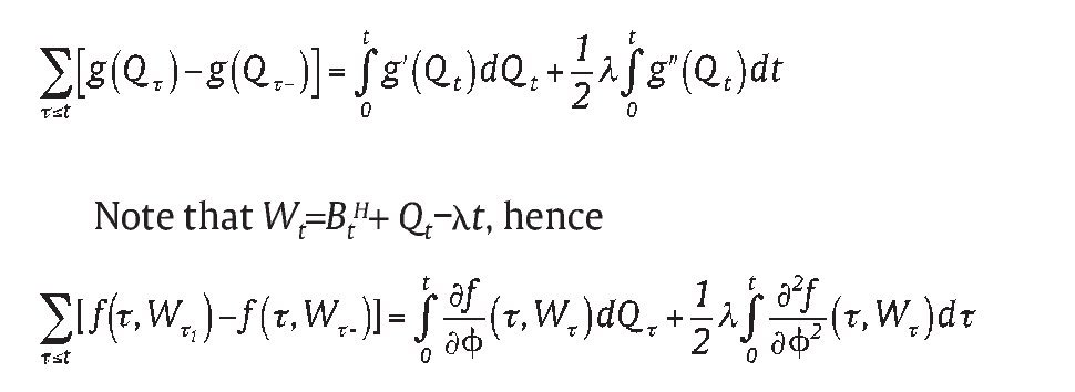
Setting ti as the jump time in the intervals [0, t] where i is the number of jump and Wt=BtH+Qt-λt. When i equal 1, using fractional Itô equation, we have
The change of f(t,Wt) at time t1 equals f(t1,Wt1)- f(t1,Wt1-) thus
Consider the number of jumps in the intervals [0, t] follows the Poisson process, hence
Say g(ϕ) ϵ C2 (R → R), and it is fact that (dQt, dQt), using the general Itô equation in g(Qt), we have,
Appendix B. Derivation of the pricing formula in corollary 1
Note that for 0 ≤ T0 ≤ t ≤ T, we can invoke the "plain vanilla" pricing formula of proposition 1.
We already know form proposition 1 that the option price at t=T0 is as follows:
where
Thus, the option price at t T 0 determined by the above formulae, i.e.:
It follows that the option price can be obtained by solving the following integral
where N is the normally distributed density function. Through some tedious algebra, we have the forward-start-averaging option formula written as Corollary 1 in the paper.
Article history: Received May 22, 2012 Accepted June 25, 2012
*Correspondingauthor.
E-mail address:
Pengbin01@hotmail.com (B. Peng); feip@ece.ubc.ca (F. Peng).
References
Alziary, B., Dechamps, J.P., Koehl, P.F., 1997. A P.D.E. approach to Asian options:
Analytical numerical evidence. Journal of Banking and Finance 21, 613-640. Bates, D.S., 1996. Jumps and stochastic volatility: Exchange rate processes implicit in deutsche mark options. Review of Financial Studies 9, 99-107.
Bayraktar, E., Poor, H.V., Sircar, K.R., 2004. Estimating the fractal dimension of the S&P 500 index using wavelet analysis. International Journal of Theoretical and Applied Finance 7 (5), 615-643.
Beckers, S., 1981. A note on estimating the parameters of the diffusion-jump model of stock returns. Journal of Financial and Quantitative Analysis 16 (1), 127-140.
Blenman, L.P., Clark, S.P., 2005. Power exchange option. Finance Research Letters 2, 97-106.
Boyle P., 1977. Options: A Monte Carlo approach. Journal of Financial Economics 4, 323-338.
Boyle P., Brodie M., Glasserman P., 1997. Monte Carlo method for security pricing. Journal of Economic Dynamics and Control 21, 1267-1321.
Chen, K.W., Lyuu, Y.D., 2007. Accurate pricing formulas for Asian options. Applied Mathematics and Computation.188, 1711-1724.
Chernov, M., Gallant, A.R., Ghysels, E., Tauchen, G., 2003. Alternative models for stock price dynamics. Journal of Econometrics 116 (1-2), 225-257.
Daly, M.T., Logan, M.I., 1998. Reconstructing Asia: The Economic Miracle That Never Was, The Future That Is. Melbourne: RMIT Publishing, Melbourne, 124-135.
Duncan, T.E., Hu Y., Pasik-Duncan, B., 2000. Stochastic calculus for fractional Brownian motion 1. Theory. SIAM J. Control Optim 38, 582-612.
Eraker, B., 2004. Do stock prices and volatility jump? Reconciling evidence from spot and option prices. Journal of Finance 59 (3), 1367-1403.
Gukhal, C.R., 2004. The compound option approach to American option on jump-diffusions. Journal of Economics Dynamics and Control 28, 2055-2074.
Harrison, J.M., Kreps, D., 1979. Martingales and arbitrage in multiperiod secutities markets. Journal of Economic Theory 20, 381-408.
Harrison, J.M., Pliska, S.R., 1981. Martingales and stochastic integrals in the theory of continuous trading. Stochastic Processes and their Applications 11, 215-260.
Hu, Y., 2003. Fractional white noise calculus and applications to finance. Infinite Dim, Anal. Quantum Probab. Related Topics 6, 1-32.
Hull, J.C., White, A., 1993. Efficient procedures for valuing European and American path-dependent options. Journal of Derivatives 1, 21-23.
Jorion, P., 1988. On jump processes in the foreign exchange and stock markets. Review of Financial Studies 1, 427-455.
Kemna, A.G.Z., Vorst, A.C.F., 1990. A pricing method for options based on average asset values. Journal of Banking and Finance 14, 113-129.
Meng, L., Wang, M., 2010. Comparison of Black-Scholes formula with fractional Black-Scholes formula in the foreign exchange option market with changing volatility. Asia-Pacific Financial Markets 17, 99-111.
Merton, R.C, 1976. Option pricing when underlying stock returns are discontinuous. Journal of Financial Economics 3, 125-144.
Neave, E., Turnbull, S., 1993. Quick solutions for arithmetic average options on a recombining random walk. In: Proc. of 4 Actuarial Approach for Financial Risks International Colloquium, 718-739.
Necula, C., 2002. Option pricing in a fractional Brownian motion environment. Academy of Economic Studies, Bucharest, Romania. Available at SSRN: http:// ssrn.com/abstract=1286833 or http://dx.doi.org/10.2139/ssrn.1286833
Pan, J., 2002. The jump-risk premia implicit in options: evidence from an integrated time-series study. Journal of Financial Economics 63 (1), 3-50.
Peters, E, 1989. Fractal structure in the capital markets. Financial Analysts Journal 7, 434-453.
Tompkins, R.G., 1999. Power options: hedging nonlinear risks. Journal of Risk 2, 29-45.
Xiao, W.L., Zhang, W.G., Zhang, X.L., Wang, Y.L., 2010. Pricing currency options in a fractional Brownian motion with jumps. Economic Modelling 27, 935-942.
Zhang, P.G., 1997, Exotic options. A Guide to the second Generation Option. World Scientific, Singapore.
Zhang, J.E., 2001. A semi-analytical method for pricing and hedging continuously sampled arithmetic average rate options. Journal of Computational Finance 5, 59-79.


