An innovative MS-VAR model with integrated financial knowledge for measuring the impact of stock market bubbles on financial security

Abstract

In the modern financial system, division of labor and close cooperation between different departments are determinants of risk contagion. The risk resulting from the volatility of the stock market can easily spread to other industries and departments, leading to systemic financial and economic crises. Previous research has mostly examined financial security from the lens of macro currency security, and the security of the banking system, but has ignored its micro-basic problems, such as the bounded rationality of investors due to the lack of financial knowledge. The study analyzes the behavior of micro-investors, price fluctuations in the meso‑stock market, and the macro-financial security in a unified framework. First, we use the comprehensive analysis method to superimpose some basic values and investor behavior characteristics, such as the stock price fluctuation index, and then construct the ultimate stock price bubble index; second, the principal component method is used to establish a financial security index that is in line with basic economic reality and consistent with previous studies; the innovative MS-VAR model is used to analyze whether the stock price bubble will affect financial security, and the rhythm and correlation of the two parties under different regimes are summarized. The results show that the stock market bubble level is the Granger cause of financial security, the stock market bubble index is the leading indicator of the financial security index, and the relevant parameters of the model are significant and have obvious economic significance. This study has important implications for scientific market regulation.

Introduction

Finance, which is the core of the modern economy, is not only an important tool for resource allocation and macro-control, but also an important force to promote economic and social development. Financial safety and stability are the basis of a country's steady and healthy economic development. Stock market risk has a micro-foundation, with some participants lacking financial knowledge and information interpretation ability. Moreover, due to the arbitrariness of transactions, irrational investors follow the trend blindly and chase sell in stock market. When stock prices rise from its basic level to the level of support, price bubbles are created, and when these bubbles reach a certain stage, they burst, and then stock prices fall rapidly, leading to sharp fluctuations in the stock market and risks in the capital market. Therefore, due to the COVID-19 pandemic, and the accelerated development of economic globalization, it is essential to improve investors’ financial knowledge, guard against capital market risks, and maintain financial security.

This study mainly analyzes the behavior of micro-investors, price fluctuations in the meso‑stock market, and macro-financial security in a unified framework, that is, the bounded rational decision-making behavior of investors due to the lack of financial knowledge at the micro level causes the excessive volatility risk of the stock market at the meso level, and the contagion effect of the risk will lead to the financial security at the macro level. The rest of this paper is organized as follows. Section 2 introduces the relevant literature and proposes hypotheses. Section 3 describes the mechanism of stock market bubbles affecting financial security. Section 4 builds a bubble index with multiple indicators that reflect the company's underlying value and market sentiment. Section 5 constructs the financial security index. Section 6 uses the innovative MS-VAR model to empirically study the impact of China's stock price bubble index on the financial security index. Section 7 presents the conclusions and makes recommendations.

Literature review

Research on stock market bubbles

The basic logic of a right-tailed unit root test (Sup ADF or SADF) and generalized right-tailed unit root test (Generalized SADF or GSADF) is to capture the nonlinear characteristics of stock prices and determine the critical value of statistics through rolling regression and forward recursion. Phillips et al. (2011) proposed SADF, which is better than ADF in the detection of periodic bubble bursts. Phillips et al.(2015)further put forward the GSADF test method, which is better suited for sequences with multiple bubbles in the sample period. Fantazzini (2016) pointed out that there was a negative bubble in the oil market in 2014–2015 by combining the GSADF method and log-periodic power model. Kraussl et al. (2016) used sup-ADF to study asset price bubbles in the art market. Liu et al.(2017) used recursive sup-ADF to study the speculative bubble of China's consumer price index from 2006 to 2014. Guo (2018) used the BSADF method to study periodic bubbles in China's stock and real estate markets, and the results showed that periodic bubbles appeared frequently during the research period. Zhang et al. (2018) used SADF and GSADF, and found that there were multiple bubbles in China's real estate market.

Ding (2021) analyzed the heterogeneity and impact of the "herding behavior" of various institutional investors under different market conditions and found that the "herding behavior" of securities investment funds and securities companies exacerbated the volatility of the stock market. Based on the monthly data for interest rates, money supply, and stock prices, Sun and Zhu (2021) studied the dynamic impact effect of price and quantity monetary policy on stock price using the MCMC method and TVP-SV-VAR model under the Bayesian framework and found that the impact of interest rates on stock prices is greater than that of money supply. Wang (2021) confirmed that the impact of monetary policy on stock asset prices is greater and lasts longer when the investor sentiment variables are included.

Research on financial security

Wang (2010) believed that capital financing secured financial security. Fredrish (2012) analyzed the types of financial systems in which financial security can be guaranteed. Emrah et al. (2013) studied the influence of financial opening on economic and financial security. The potential risks of the capital market have an impact on financial security (Zhu & Zhang, 2017). Liang (2018) analyzed the mechanism of systemic financial risks from the theoretical level and evaluated China's financial security from both macro and micro perspectives. A sovereign credit rating is related to a country's financial security and stability (Li, 2019). Zhao (2020) proposed the principles of effective supervision of legal digital currency risks, active maintenance of financial security, promotion of financial innovation, and development of regulatory technology. Excessive debt can easily lead to systemic risks, which is not conducive to maintaining financial security (Li & Ning, 2020). Miao and Run (2020) studied and proposed prevention suggestions based on three aspects, namely, the measurement method of systemic financial risk, risk contagion effect, and selection of regulatory tools. The impact of interest rate shocks and interest rate fluctuations on financial security is strongest during an economic crisis and weak during the period of the economic new normal (Liu et al., 2021).

Research on financial knowledge

Noctor et al. (1992) first proposed the concept of financial knowledge, which is defined as people's ability to make wise judgments and effective decisions in the use and management of funds. Lusardi et al. (2014) defined financial knowledge as the information related to people's handling of economic and financial affairs and the making of reasonable decisions in terms of wealth accumulation, financial planning, debt planning, investment management, and so on. Wu (2015) believed that the popularization of financial knowledge was an effective way to improve the breadth and depth of financial product investment. Xiang and Guo (2019) found that financial knowledge can change investors' risk attitudes. Jia (2020) found that popularizing financial knowledge helped to reduce the ratio of retail investors in China's stock market and promote the development of institutional investors. Gong et al. (2021) studied the interaction between heterogeneous traders and their impact on price discovery by establishing a futures market pricing model and found that behavioral factors, such as risk appetite, rationality, and market liquidity had a comprehensive impact on stability conditions. Xie (2021) believed that increasing the popularity of financial knowledge can significantly improve the level of human capital accumulation, restrain financial risks, and subsequently reduce the distortion of market factors. Luo (2021) found that financial knowledge can boost household consumption spending by improving the structure of household financial asset allocations.

Mechanism of stock market bubbles affecting financial security

Impact of investor behavior on stock price

• (1)

  Influence of investors' bounded rationality on stock price

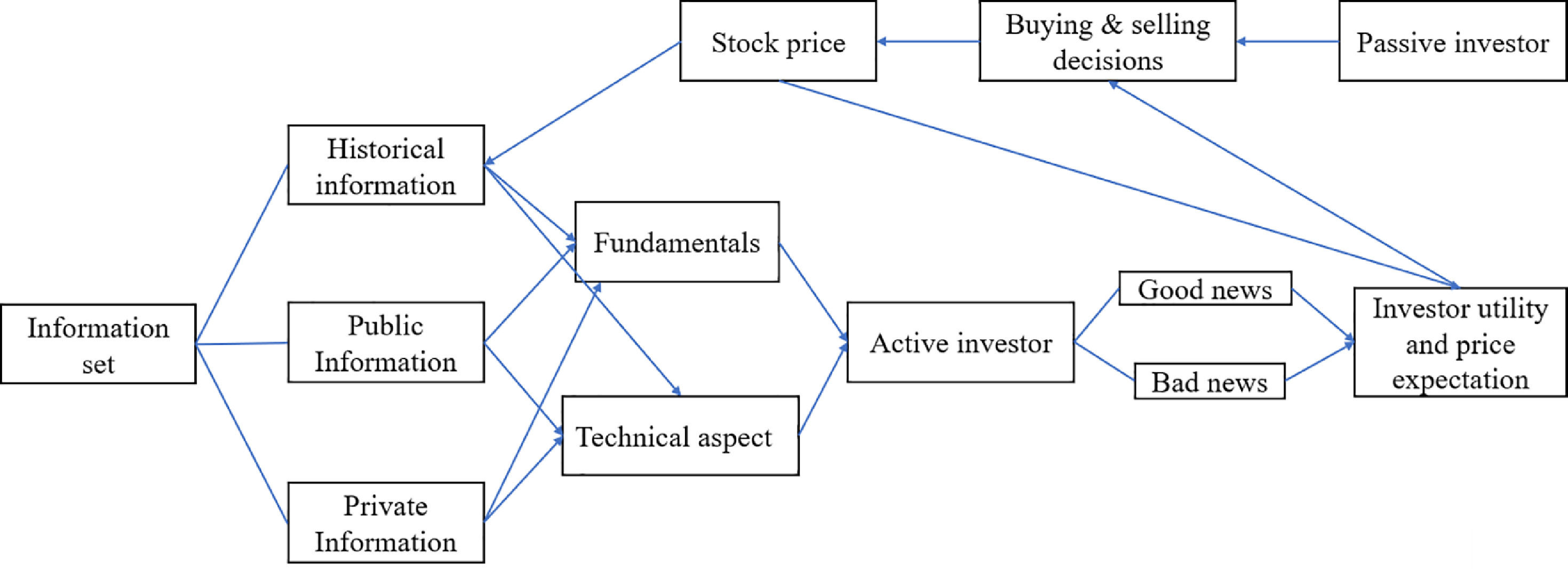
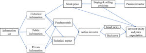
Given the influencing factors of stock price, Fama (1970) presented the efficient market hypothesis (EMH), which holds that from the perspective of information economics, the stock price is determined by and responds to information. The EMH theory is only a theoretical abstraction and simplification of the real price determination process because information cannot automatically affect the price and because investors, a key factor, are ignored. The premise for the information to work is that there are investors in the market who receive and interpret relevant information to form good and bad expectations regarding fluctuations in stock price. Under this expectation, buy and sell decisions are formed, and the purchase and sale orders of all investors in the whole market are gathered to form the equilibrium price of the stock at a certain time.

As shown in Fig. 1, the stock price formation process can be described as follows: investors classify all information (historical, public, and private information) into two types: fundamental and technical information. Then, they interpret it as good or bad news regarding the corresponding stocks and form stock price expectations through the investor utility function. Subsequently, purchase and sale decisions are made, and finally, stock prices are determined. From a dynamic point of view, the newly formed stock price directly affects investors' expectations and is considered new historical information, becoming the basis for further analysis by investors.

Fig. 1.

Information, investor expectations, stock price transmission chain.

Considering investors as the research object may more truly reflect the trading situation in the stock market and the stock price decision process. Moreover, investors’ bounded rationality and investor sentiment have naturally appeared in the field of vision as new research dimensions. In the traditional rational person hypothesis, investors' processing of all kinds of information is unbiased and cost-free. If we ignore this hypothesis, that is, investors are limited rationally and cannot interpret all kinds of information accurately, the biased behavior of investors will evolve into market sentiment, resulting in investors making too optimistic or pessimistic judgments about stock price. The stock market is prone to price bubbles as they are greatly affected by investors' behavior bias. Therefore, investor behavior is one of the important factors that determine stock price.

• (1)

  Influence of financial knowledge on stock market investment

Investors' bounded rationality will be manifested in various belief and behavior deviations, including loss aversion, regret avoidance, overconfidence, lack of self-confidence, and herding behavior. Generally, the bounded rational behaviors of these investors accumulate in the stock market, resulting in a high stock turnover rate, soaring stock prices, and other phenomena, which can be summarized as the emotional factors that determine stock price.

Financial knowledge affects investor participation in the stock market in many aspects. First, investors with financial knowledge can identify the risks and benefits of various stock products and reduce the threshold for entering the stock market. Second, with improvements in investors' financial knowledge, their acceptability of risk will also be enhanced, and their interest in investing in the stock market and choosing high-risk investment types, such as stocks will also be greatly promoted. Third, when investors have rich financial knowledge, it is not easy to produce cognitive biases, such as overconfidence. They focus more on allocation to different kinds of assets in accordance with their risk preference to ensure that they do not blindly pursue high returns and put all their assets in risky investments such as stocks, leading to the emergence of stock price bubbles (SPBs). Finally, further improvements in financial knowledge enable investors to reduce transaction costs and hold a more reasonable and effective portfolio.

Analysis of the concept of financial security and its influencing factors

• (1)

  Definition of financial security

Financial security is mainly defined from three angles: the financing security of monetary funds, the security of national interests, and the security concept of financial risk and crisis. Considering the literature, we define financial security as the state of healthy, stable, and orderly development of the financial industry. In this state, financial risks are controllable and do not accumulate above the threshold, resulting in no financial crises.

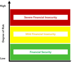
The security status of the financial system can be described as a three-zone system, as shown in Fig. 2: Financial security (green), indicating that the risk of the financial system is controllable and operates well; Financial insecurity (mild, yellow) means that there is some accumulation of financial risks, and if the risk continues to accumulate it will threaten the stability of the financial system. Regulatory authorities need to deal with it in a timely and correct manner, to reduce financial security risks, or to at least maintain a mild state of financial insecurity and prevent further deterioration. In a state of financial insecurity (serious, red light), there will generally be a financial crisis, and once the risk breaks out, regulatory authorities need to take measures to deal with it quickly.

• (1)

  Definition of financial security

Fig. 2.

Schematic diagram of the security status of the financial system.

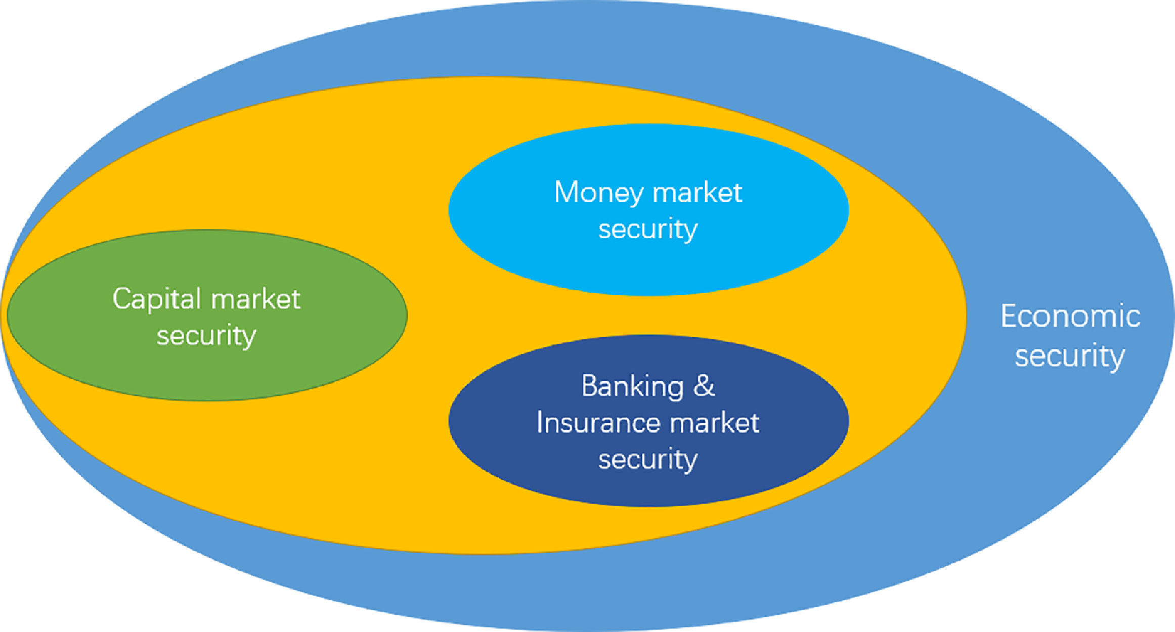
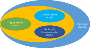
The financial system is complex and huge, and according to the current supervision mode of China's financial industry, it includes at least the following three subsystems, as shown in Fig. 3: Banking and insurance subsystem, securities subsystem, and currency subsystem. At the same time, from a broader perspective, the financial system is also a subsystem of the economic system, and the security of economic operations is essential for the security of the financial system. Therefore, the influencing factors of financial security can be analyzed from four dimensions: economic system security, banking and insurance system security, capital market security, and monetary security.

Fig. 3.

Schematic diagram of the factors affecting the financial security system.

Path analysis of stock market bubbles affecting financial security

From the analysis in the previous section, it is evident that banking and insurance industry security, capital market security, and money market security are the three subsystems of the national financial security system. The security and stability of the stock market directly affect the security and stability of the capital market which subsequently affects financial security. The periodic expansion and rupture of stock market bubbles are typically unsafe events in the capital market, especially when stock prices collapse due to the bubbles bursting, and the effect of the collapse is transmitted and spread through the mechanism of the enterprise/family balance sheet effect. This leads to corporate liquidity risks and banking and currency crises, which ultimately affect financial security. The mechanism of the stock market bubble's impact on financial security can be divided into the family balance sheet effect and enterprise balance sheet effect, and after superimposing the principle of the financial accelerator, the corresponding impact effect is amplified.

• (1)

  Household balance sheet effect

In the SPB expansion stage, individual investors with limited rationality will constantly revise their expectations, their emotions will become increasingly more optimistic, the effect of virtual wealth will be stronger, the level of consumption will improve, and consumption expenditure will be increased by mortgage. Thus, in the bubble burst and stock price collapse stage, the effect of wealth deflation will be significant, the shrinking of virtual wealth in the hands of investors will inhibit consumption expenditure, reduce total social demand, and slow economic growth. Some investors with leveraged consumption will default due to cash flow problems, and the crisis will extend to banks and other financial sectors.

• (1)

  Enterprise balance sheet effect

The decline of the stock market worsens the balance sheet of enterprises, as the value of assets decline but the value of liabilities do not. To alleviate the debt pressure, enterprises usually need to sell equity in the secondary market, which further causes a decline in the stock market. If the debt type of the enterprise is an equity pledge, the decline in share price will lead to an insufficient value of the equity pledge, and financial institutions, such as banks or securities companies, will require an increase in the pledge. When the enterprise cannot take out the full amount of the pledge, the pledged equity may be sold, resulting in a sharp decline in share price and the demonstration effect of the decline. Severely insolvent enterprises will go bankrupt and liquidate, and the existence of mutual guarantee mechanisms for enterprise financing from banks will simultaneously lead to continuous debt default, which will induce the risk of asset losses in banks and other financial sectors, and the crisis will continue to spread, ultimately affecting financial security.

• (1)

  Principle of the financial accelerator

There is a negative correlation between the agency cost of external financing and the borrower's net asset value. Therefore, if the borrower's net asset value changes positively with the economic cycle (e.g., when enterprises’ profit and asset price increase with the economic cycle), the agency cost of external financing will change inversely with the economic cycle. Especially in periods of economic recession, the external financing cost of enterprises continues to rise, resulting in the contraction of enterprises' investment, expenditure, and production activities, and the contraction further triggers a new round of adverse shocks, which continue to strengthen and cause an economic recession. This impact amplification effect is the principle of the "financial accelerator". It can be said that the superimposition of the financial accelerator effect and balance sheet effect is the internal mechanism of the diffusion of most financial crises in various social and economic sectors (Bernanke & Ben, 1983; Bernanke & Gertler, 1989; Bernanke et al., 1996).

Construction of the stock market bubble index

Tobin's Q value method and K bubble coefficient method are characterized by a single index, which is simple but the degree of disclosure is not enough from the consistency of research methods and practicality perspective. The GSADF method simply studies the existence of bubbles from the stock price perspective itself but does not accommodate basic factors and investor sentiment factors. However, due to the comprehensive consideration of the basic value and emotional indicators, the price bubble index obtained by the principal component method is more appropriate to reveal the degree of the market bubble. Therefore, this research method is adopted in the analysis of the impact of bubbles on financial security.

Basic models

• (1)

  Principal component model

The core idea of principal component analysis lies in dimensionality reduction to simplify the problem, which can help to extract most of the information regarding the original variables when performing multivariate analysis where correlation exists and the information is not duplicated (Dai & Deng, 2018). The key to principal component analysis is to determine the loadings of the original variables on the plural principal components.

Where, ai1,ai2…aij(i=1,2,…p) represent the eigenvector corresponding to the eigenvalue of the covariance matrix of variable. x,x1,x2,…,xp represent the value of the original variable after standardization. The standardization of original variables is due to the inconsistency of the original data index units, and there is a biased influence of the dimensions on the statistical analysis results. Therefore, standardization is needed to eliminate dimensional factors and ensure that the analysis results are accurate.

Determination principle of coefficient aij:

First, yi and yj (i≠j; i, j = 1, 2, …, m) are independent of each other. Second, y1 has the largest variance in all linear combinations of x1,x2,…,xp, and y2 has the largest variance in all linear combinations of x1,x2,…,xp not related to y1,yp has the largest variance among all linear combinations of x1,x2,…,xp that are not related to y1,y2…,ym−1 The new variable index y1,y2,…,yp is called the first, second, ….and P principal components of the original variable index x1,x2,…,xp.

• (2)

  State-space model and the Kalman filter algorithm

State-space models arise from the analysis of smooth time series and portray the dynamic change process of variables. The Kalman filter algorithm is a data processing technique of removing noise to restore real data and is easy to implement programmatically. It was initially used in engineering and is now increasingly used in the analysis of economic problems. The linear factor spatial state model is established based on relevant variables:

Where wt∼N(0,Q) is the process noise, et∼N(0,R) is the measurement noise, Xt is the state variable, Yt is the output vector, A is the transfer matrix, B is the output matrix, and the initial state of the system is X0, the mean value is μ0, variance is Σ0, and the covariance is COV0.

In the state-space model of dynamic systems, the system state vector X1:n=[X1,X2,…,Xn] is unobservable, and the observable measurements are vector Y1:n=[Y1,Y2,…,Yn] and parameter set Θ=[A,B,Q,R,μ0,COV0], the Kalman filter method is used to estimate X1:n which is based on known Y1:nand Θ. Assuming that the noise obeys the normal distribution, the mean Xt|t=E(Xt|Y1:t) and covariance COVt,t|t=COV(Xt,Xt|Y1:t) of the probability estimation at time t can be estimated by the parameters Xt−1|t−1 and COVt−1,t−1|t−1at time t-1. According to Thomas (2005), the main results are as follows:

Indicator selection

The results of indicator selection and its basic logic are:

• (1)

  Average price-to-earnings ratio (P/E) of SSE A-shares

• (2)

  Total market capitalization-weighted monthly market turnover ratio (TTR)

• (3)

  Stock turnover amount (R): The absolute value of the turnover amount is more ambitious, and the current month's year-on-year data is used here

• (4)

  Number of shares traded (M): This indicator also uses month-on-month data

• (5)

  Total stock market capitalization on SSE (N): Using month-on-month data

To eliminate the effect of dimensionality, the stock volume is unitized and a total of five variables, PE, TTR, R, M, and N, are used. The original data are monthly data except for GDP, which is quarterly data. In this study, the cubic-match last method provided by EViews software is used to increase the frequency of GDP data.

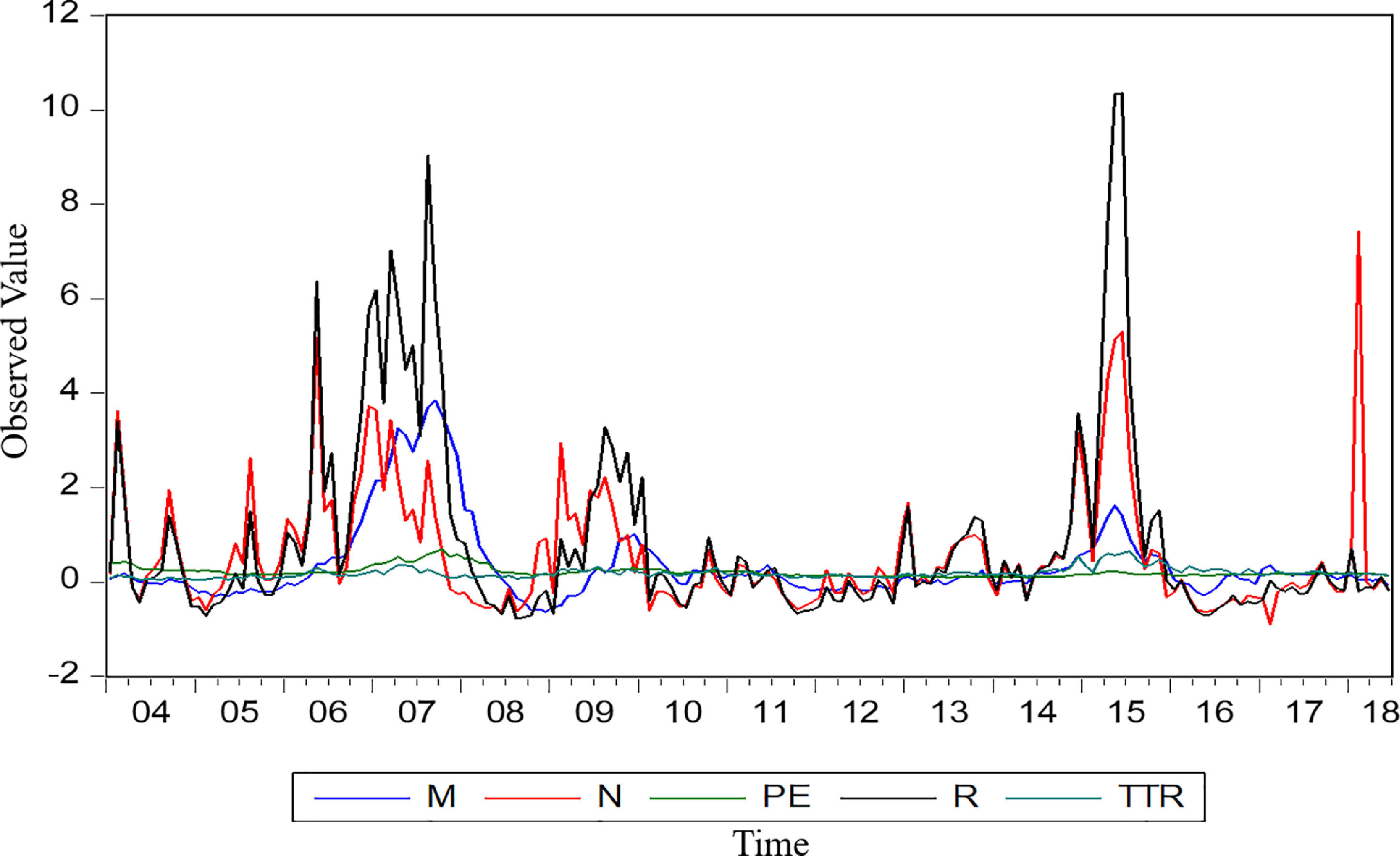
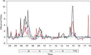
Descriptive statistics

Fig. 4 shows the sequence diagram of five basic variables. These indicators have a certain collinearity, which is suitable for analysis using the principal component method. According to the results of descriptive statistics (Table 1), it can be found that the mean, maximum and minimum values of the stock market turnover ratio, P/E ratio, M, R, and market trading volume all vary widely, which shows that the stock market in China changes more drastically, and this unstable characteristic can easily create a bubble in the stock market. The skewness of each indicator is greater than 0, which is right-skewed, and the largest Kurtosis value is the series R. However, the remaining indicators are not seen below 7, which shows that the probability distribution expressed by the sample data slightly deviates from the normal distribution and is positively skewed (or right-skewed) and has a fat-tailed distribution.

Fig. 4.

Sequence diagram of five basic variables.

Table 1.

Data descriptive statistics.

	M	N	PE	R	TTR
Mean	0.354963	0.591828	0.211805	0.895911	0.187488
Median	0.10705	0.16355	0.17665	0.10335	0.162498
Maximum value	3.8421	7.422	0.6964	10.3485	0.649182
Minimum value	−0.629	−0.8959	0.0976	−0.7839	0.041519
Standard deviation	0.840133	1.288658	0.112101	2.04715	0.109258
Skewness	2.440913	2.199361	2.02122	2.458817	1.835588
Kurtosis	8.79661	9.086048	7.150209	9.483288	7.311311

Principal component analysis method

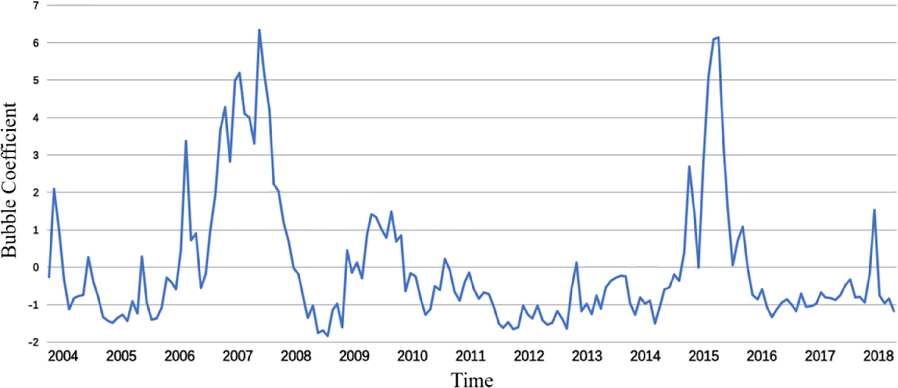
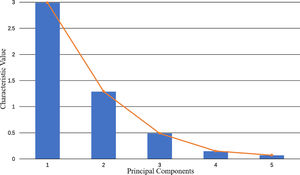
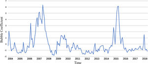
The five variables are standardized and the principal components are selected by a principal component analysis (Table 2). The cumulative contribution of the first two principal components is 85.55%, which exceeds the standard level of 85%, and the gravel plot (Fig. 5) produces a visible turn at the second point. Therefore, the first two principal components are selected as representatives of the market bubble level and used to construct the stock bubble index. Based on the extracted principal component common factors, the SPB coefficient can be constructed as shown in Fig. 6.

Fig. 5.

The scree plot of principal component analysis.

Fig. 6.

Schematic diagram of the stock price bubble coefficient trend.

Kalman filter algorithm

To remove the influence of clutter, the SPB index is optimized by constructing a state-space model and using the Kalman filtering algorithm. First, the spatial state model of the five indicators and the stock bubble index is established, the dependent variable is denoted as PAC, the fixed regression coefficient variable is C, the five indicators are all regression variables with AR (1) random coefficients, and the underlying variance structure is a general diagonal matrix (diagonal). The established measurement equations and state equations are:

Measurement equation:

Equation of state:

Second, estimating the state-space model using the Kalman filter algorithm requires specifying the initial values of the unknown parameters (hyperparameters). The initial values of c(1), and c(2) can be obtained by establishing the following regression equations.

The intercept term C (1) of the reference regression equation is −1.9758, and the parameter C (1) of the set state equation is also taken as this value. The residual sum of squares (RSS/T) of the equation is taken as an estimate of the variance, and its logarithm is obtained as C (2) = LOG (143×10−19/174) = −19.08521321. The valuation of C (3)-C (15) is estimated as follows. By modeling state space with each of the five indicators, a regression equation is established and the two unknown parameters of the measurement equation are estimated according to the intercept term and residual sum of squares. According to Gao et al. (2016), the three unknown parameters of the state equation can be first assigned as 0.1, 0.9, and −9. Then, the estimated values of the two parameters of the above measurement equation and the initial values of the three parameters of the state equation are inputted using the param command, and the state vector obeying AR (1) is predicted. Finally, the three unknown parameters of the state equation are determined by building the estimated coefficients of the AR (1) model of the state vector and the residual sum-of-squares estimation, where C(3n) =log (RSS/T), n = 1, 2…5.

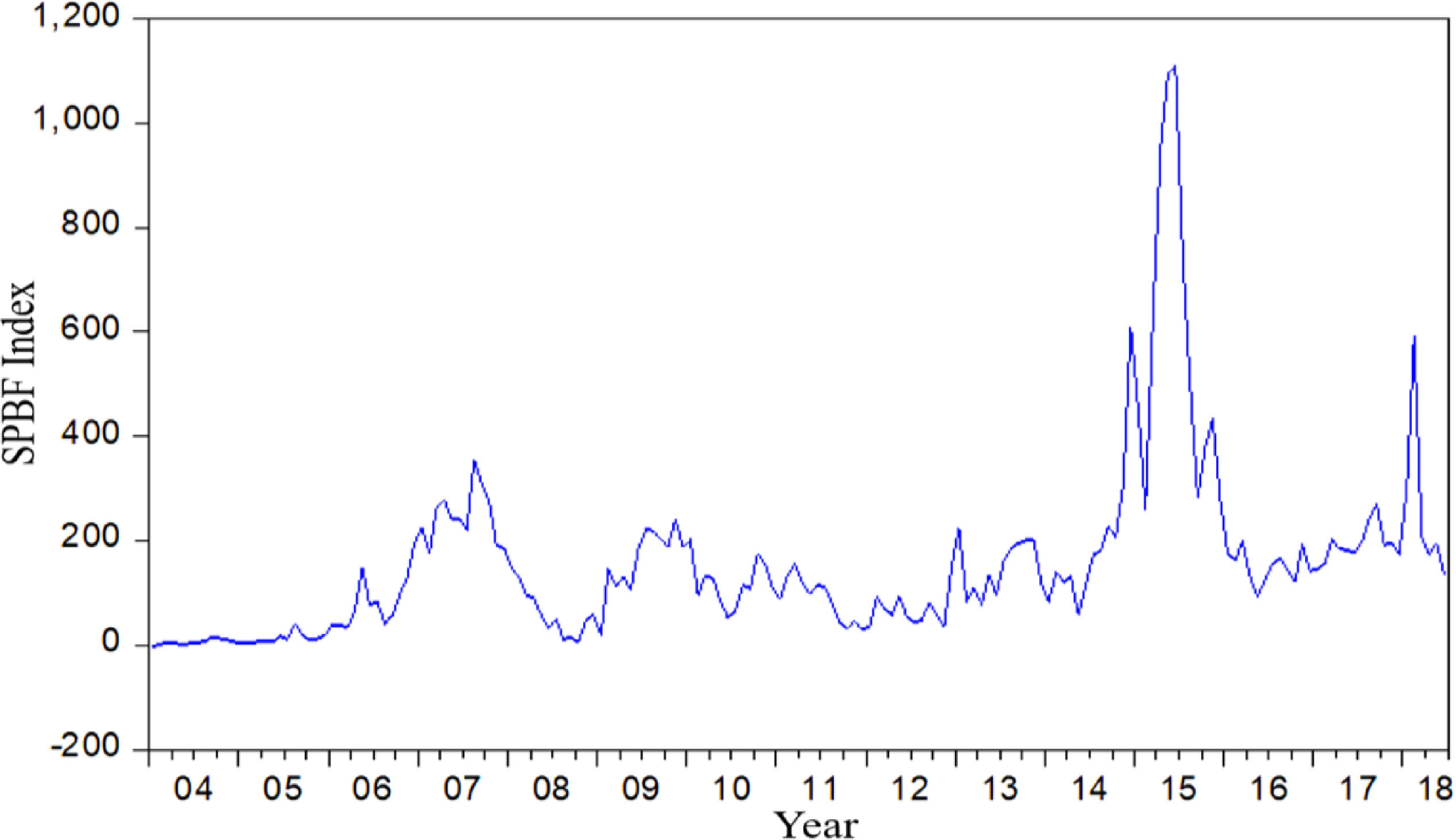
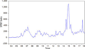
After the above optimization of the SPB index by applying the Kalman filter algorithm, the SPBF index (Fig. 7) can be obtained as the final measure of the size of the stock market bubble.

Fig. 7.

Schematic diagram of the stock price bubble coefficient optimized by Kalman filter.

Fig. 7 shows that China's stock market has experienced severe bubbles during the four periods of 2007, 2009–2010, 2014–2015, and 2017, which is consistent with the actual market trend. Moreover, the bubble index shows that the bubble level of the stock market during the 2014–2015 period is higher than that of the 2006–2007 period, which reveals the actual situation of the A-share bull market in the 2014–2015 period. Thus, the index of the constructed SPBs not only synchronizes with the sharp rise and fall of the stock market, but also reveals the extent of support of the real economy in a rising stock market, and further confirms that the selected principal component index can better measure the size of the stock market bubble.

Construction of the financial security index

In this section, we discuss the construction of China's financial security index based on principal component analysis. He and Lou (2012) selected 26 indicators for principal component analysis from four dimensions: micro-financial institution security, meso‑financial-market security, macroeconomic operation security, and international external risk impact. Jia and Li (2015), and Liang (2016) selected 16 indicators from the 2 dimensions of the macroeconomic environment and financial industry evaluation for principal component analysis. Liang et al. (2018) selected 23 indicators from the 4 dimensions of the macro economy, capital market, money market, and foreign exchange market for principal component analysis. Guo et al. (2018) used the factor analysis method based on panel data to construct China's regional financial security index by region and identified the status of China's regional financial security in different periods based on the MS-VAR model. Xu and Zhou (2019) used principal component analysis to estimate the financial security index from 2000 to 2016 and analyzed the impact effect of macroeconomic fluctuations on financial security. Gu et al. (2020) constructed a financial security assessment system based on the three perspectives of macro-level, fiscal level, and financial level, and analyzed China's overall financial security and the financial security of the four economic regions by using the entropy method. Zhou et al. (2021) selected 22 mixing sample data composed of annual, quarterly, and monthly frequencies, estimated them using the newly constructed mixing layered dynamic factor model, and measured China's mixing financial security index system.

In the literature, the principal component method is the main method used to construct the financial security index. The idea is to simplify multiple interrelated basic indexes into a few comprehensive indexes through dimension reduction technology. Moreover, these few comprehensive indexes are not related to each other, and they can provide most of the information of the original indexes. With the process of principal component analysis, the weight of each principal component is generated automatically, which largely offsets the interference of human factors in the evaluation process. Therefore, the comprehensive evaluation theory based on principal components can better ensure the objectivity of the evaluation results and truthfully reflect the actual problems.

Design ideas of the financial security index

• (1)

  Design ideas

The financial industry has its particularity in product supply and pricing of mainly virtual assets, where the prices are highly volatile. The influencing factors of financial system security can be analyzed from four dimensions: economic system security, banking, and insurance system security, capital market security, and currency security. Among them, economic security is the macro background of financial security. Banking and insurance security, capital market security, and currency security are subsystems of financial security. This division standard completely covers all the influencing fields of financial security. Therefore, following this logic, in this section we take these four dimensions as the first-level indexes, and establish the second-level and third-level indexes accordingly, to construct a more reasonable and reliable financial security index. The availability of data should be considered in the construction of indexes, as shown in Table 3.

The first-level index to describe the degree of financial security should be referred to by the four systems, namely, the macroeconomic system, banking and insurance system, capital market system, and monetary system. Each first-level index is divided into second-level indexes that can describe its basic operation status. For example, the macroeconomic system can take economic operation status and financial policy status as second-level indexes; the banking and insurance system can be naturally decomposed into two second-level indexes: the operation status of banking and insurance; the capital market consists of the stock market, bond market and derivatives market. Considering the market scale and influence, only the stock market is introduced as the second-level index; the money market considers the internal and external value of money as second-level indexes.

In terms of third-level indexes, the economic operation of the macroeconomic environment can be tracked by the GDP growth rate, fixed asset investment growth rate of the whole society, and the macroeconomic prosperity leading index; financial policy can be represented by the year-on-year growth rate of M2; the third-level indexes of banking operation can include the non-performing loan ratio of commercial banks and the monthly standard deviation of the interbank 7-day lending rate; the third-level indexes of the insurance industry include the growth rate of insurance assets and the growth rate of insurance total compensation; the monthly standard deviation of the Shanghai Composite Index is introduced to measure the third-level indexes of the stock market; indexes of currency security include the CPI and the monthly standard deviation of exchange rates between the US dollar and RMB. There are 11 economic indexes.

• (1)

  Description of indicators

• ① GDP growth rate: The GDP index is the background of the whole financial security problem; hence, it must be selected.

• ② CPI: CPI is selected to reflect the overall price level.

• ③ Leading index of macroeconomic prosperity: A low index indicates that a country's economy has downward expectations, and vice versa.

• ④ The growth rate of fixed-asset investment in the whole society: Investment is one of the important factors driving China's economic growth; therefore, the growth rate of fixed-asset investment in the whole society can be used to reflect the contribution of investment to China's economic growth and the stability of China's financial system.

• ⑤ The M2 year-on-year growth rate: This indicator reflects a country's macro-financial environment.

• ⑥ The monthly standard deviation of USD/RMB exchange rate: This indicator reflects the fluctuation risk of the exchange rate, the greater the volatility, the greater the overall uncertainty risk of the financial industry.

• ⑦ The monthly standard deviation of the 7-day interbank offered rate: This represents the volatility of the income level of the money market and reflects the changes in the supply and demand of short-term funds in the market. If the fluctuation range of the interbank rate offered increases, the risk of the financial industry increases, which is a reverse indicator of financial security.

• ⑧ The growth rate of insurance assets: The larger the index, the larger the scale of the insurance industry. The overall anti-risk ability is enhanced; therefore, this index is the same direction index of financial security.

• ⑨ The growth rate of total compensation in the insurance industry: This index is inversely proportional to the profit margin of the insurance industry, the higher the index, the more is the profit level of the insurance industry affected.

• ⑩ The non-performing loan ratio of commercial banks: This is an important indicator that reflects and evaluates the status of bank assets.

• ⑪The monthly standard deviation of the Shanghai Composite Index: The standard deviation is used to indicate the size of market fluctuation. If the standard deviation of the Shanghai Composite Index becomes larger, it indicates that the financial market risk increases.

Empirical analysis of financial security based on principal component analysis

• (1)

  Data selection and processing

The first step is the direction processing of data: According to the positive and negative correlation between the financial security index and selected indexes, positive correlation indexes, such as GDP growth rate, retain the original data; the negative correlation index can be transformed into the positive correlation index by equation X*=100%-X or X*=1/X. The second step is the standardization of data: The Z-value method is used to standardize data.

• (1)

  Results of empirical analysis

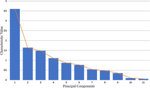
According to the principle of availability, we select 11 indexes to calculate the financial security index (Table 4), where each index has 174 observed values (January 2004-June 2018). Table 4 presents the results of the principal component analysis. It shows that the eigenvalues of the first 5 principal components are close to 1, and the cumulative variance contribution rate of the first 5 principal components is 79.08%, which shows that these 5 principal components contain nearly 80% of the information of all indexes and have good representativeness for all indexes. As can be seen from the gravel diagram in Fig. 8, the eigenvalues of the first 5 principal components change significantly, and then they are relatively gentle. Therefore, we select the first 5 principal components to replace the original 11 indexes.

Fig. 8.

Scree plot of principal component analysis.

KMO test and SMC test were performed on the above analysis, and the results are as shown in Table 5. A KMO test is used to measure the correlation between variables, and the value is between 0 and 1. The larger the value, the stronger the correlation between variables. SMC is the square of the complex correlation coefficient between a variable and other variable, and the higher the value, the more suitable the principal component analysis. In Table 5, the test results meet the requirements, indicating that it is suitable for principal component analysis.

Next, we calculate the factor load matrix. Table 6 shows that the absolute value of the load coefficient of CPI (year-on-year in the current month), GDP (year-on-year in the current quarter), the 7-day weighting of interbank lending, and the macroeconomic prosperity index (leading index) in the first principal component expression is the largest, indicating that the first principal component can comprehensively reflect these four indexes. The absolute value of the load coefficient of fixed asset investment (year on year in the current month), M2 (year-on-year), and the macroeconomic prosperity index (leading index) in the second principal component expression is the largest, indicating that the second principal component can comprehensively reflect these three indexes. In the third principal component, the absolute value of the load coefficient of the monthly standard deviation of the central parity of the US dollar against the RMB is the largest. In the fourth principal component, the absolute value of the load coefficient of the proportion of non-performing loans (Commercial Banks) is the largest. In the fifth principal component, the absolute value of the load coefficient of the monthly standard deviation of the Shanghai Composite Index is the largest.

In conclusion, the first principal component mainly represents the macroeconomic operation, and the second principal component mainly represents the financial policy, both of which belong to macroeconomic system security factors. The third principal component can be called the currency security factor, the fourth principal component is the safety factor of the banking and insurance industry, and the fifth principal component is the security factor of capital markets. The results of this principal component analysis cover the four dimensions of financial security influencing factors, which are general and representative.

According to the factor score coefficient matrix shown in Table 7, the score s1,s2,s3,s4,s5 of five principal components in each year can be calculated with the following formula:

x1,…,x11is the index value of 11 original indexes after standardization.

We take the weighted average of the scores of the first five principal components, and calculate the comprehensive evaluation scores of each year, expressed in S. The weight is the variance contribution rate of the principal components, and the formula is:

Then, the calculated value S is normalized to the interval [0, 100], the financial security index can be obtained, and the calculation formula of conversion is:

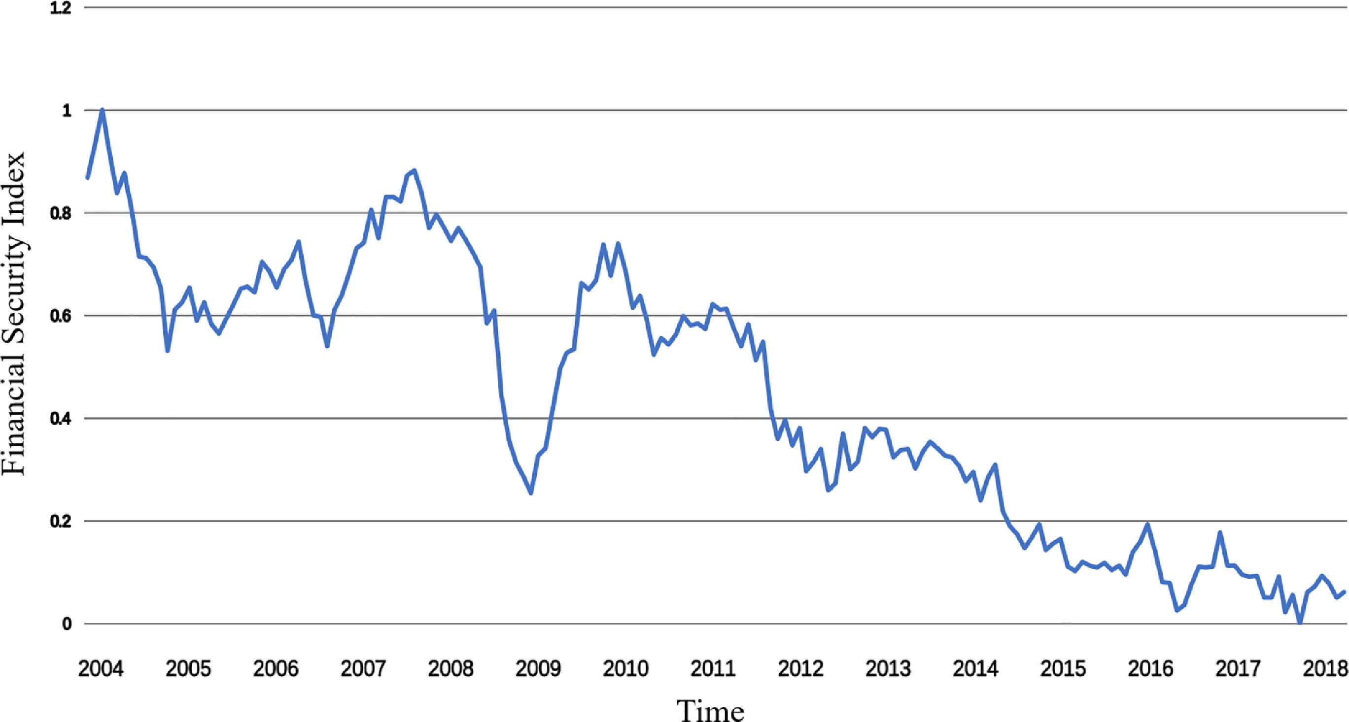
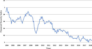
From the fluctuation trend in Fig. 9, we can see that China's financial security index has roughly experienced five fluctuations in the same direction during the sample period, namely, the continuous decline from January 2004 to July 2005, the improvement of shocks from August 2005 to October 2007, the decline from November 2007 to February 2009, the improvement from March 2009 to February 2010, and the continuous decline since March 2010. The performance of the financial security index at each stage is driven by the main economic indicators and has a profound economic background.

Fig. 9.

Financial security index in China (January 2004 - June 2018).

Impact of stock market bubbles on china's financial security

Basic principle of the innovative MS-VAR model

In this section, we empirically study the impact of China's SPB index on the financial security index by using the innovative MS-VAR model, to find evidence of the interaction between the two parties from real market data. The innovative MS-VAR model is based on the traditional VAR model and adds the Markov regime transfer model, which better describes the nonlinear time-varying characteristics of financial time series. Moreover, it can automatically divide the data into different zones according to the instructions and can discuss the influence process and effect under different zones. Hamilton (1994) first used the nonlinear Markov system transformation model to study the volatility of real output growth in the United States. Brooks and Karasaris (2005) also applied the MRS model to study the stock market bubble problem; Wang and Wang (2016) used this model to study China's financial stress index composed of currency, bank, and asset bubble risks and analyzed the market risk situation. The Markov regime transfer autoregressive model can avoid information loss and the risk of subjective judgment error, and determining the risk interval and threshold in advance is not necessary. Its use can be given priority in the research of financial security early warnings (Shen et al., 2019).

Innovative MS-VAR (P) with a delay of p order is expressed as:

Where stis the unobservable regime, the transformation probability from regime i to regime j is:

Where m represents the number of regimes, assuming m = 3, then the corresponding probability transformation matrix is:

For any i∈{1,2,3}, there is pi1+pi2+pi3=1.

Assuming that the mean, variance, intercept, and coefficients of the equation can be changed, various innovative MS-VAR models can be obtained. For the three regimes system, the mean and variance of the adjusted innovative MSMH (3)-VAR (P) model with lag p order can be written as:

Of which u(st) represents the mean value under different regimes, ut∼NID(0,∑(St)). When st=1, u(st)=u1; When st=2, u(st)=u2; When st=3, u(st)=u3. It can be seen from Eq. (9) that a change in the regime will lead to a jump in the mean value. It may be more accurate to assume that the mean value reaches a new level after the conversion from regime i to regime j. The intercept and variance-adjusted innovative MSIH (3)-VAR (P) model of the three regimes lag p-order can be expressed as Eq. (10):

Where v(st) denotes the intercept under different regimes, vt∼NID(0,∑(St)). When st=1, v(st)=v1; When st=2v(st)=v2; When st=3, v(st)=v3.

Empirical analysis based on innovative MS-VAR model

• (1)

  Determining the lag order of the innovative MS-VAR model

First, the financial security index (PAC) discussed in Section 5 and the stock market bubble index (BUBBLE) discussed in Section 4 are tested for stationarity and Granger causality. Subsequently, the lag order of the innovative MS-VAR model is determined using EViews software. The sample range is 174 months from January 2004 to June 2018.

According to the ADF test, the unit root test is carried out on PAC and BUBBLE. The test results are shown in Table 8: the BUBBLE is a stationary sequence at the 1% significance level, and the PAC is a stationary sequence at the 1% significance level after the first-order difference, which is a first-order mono-integral at the 1% significance level.

The Granger causality test is carried out on the stable first-order differential financial security index (DPAC) and BUBBLE (the data volume is reduced to 173 periods), and the results are shown in Table 9. The test results show that we accept or reject the original hypothesis that the financial security index is not the cause of the stock market bubble index under the 5% significance level. This shows that there is a unilateral Granger causality relationship between the stock market bubble index and the financial security index, that is, the change in the stock market bubble index can be used to explain the change in the financial security index.

EViews software is used to determine the lag order of the innovative MS-VAR model. The results are shown in Table 10. When the model lag phase is in the third order, the likelihood ratio test (LR) value of VAR model is the largest, and the final prediction error final prediction error (FPE) value is the smallest, and the value of Akaike information criterion (AIC) is the smallest. Generally, if the test results are inconsistent, the AIC shall prevail. In this test, compared to other lag orders, lag order 3 concurrently fulfills the principles that the minority obeys the majority and the secondary obeys the main. Therefore, we choose to establish VAR model with lag order 3.

• (1)

  Determining the number of model regime states

To study the impact of stock market bubbles on financial security, it is necessary to determine the optimal number of financial security regimes. The state of financial security can generally be divided into three states: financial security (green), financial insecurity (mild/yellow), and financial insecurity (serious/red). Therefore, we build a three-regime innovative MS-VAR model. According to whether the intercept, variance, and mean value of the innovative MS-VAR model change with the state concurrently, a model with different parameters that changes with the state can be constructed. VAR (3), MSM (3)-VAR (3), MSI (3)-VAR (3), MSMH (3)-VAR (3), MSIH (3)-VAR (3), and MSIAH (3)-VAR (3) are established, respectively, as shown in Table 11, and then the parameter morphology of the innovative MS-VAR models is determined according to AIC, HQ, SC rules, and logarithmic likelihood value LL.

It can be seen from Table 11 that according to AIC, HQ, and SC criteria, the innovative MS-VAR model with the three regimes system and third-order lag is superior to the traditional linear VAR model, and the MSIH (3)-VAR (3) model in the innovative MS-VAR model is the best in terms of AIC, HQ and SC. The linear test value LR of this model is 136.4123, and the P-value of chi-square statistics is 0, which shows that the fitting effect of the innovative MSIH (3)-VAR (3) model is the best. Therefore, the innovative MSIH (3)-VAR (3) model will be used in the follow-up empirical test.

• (1)

  Parameter estimation of the innovative MSIH (3)-VAR (3) model

The OX-MSVAR package of the Givewin platform is used to estimate the parameters of the innovative MSIH (3)-VAR (3) model, and the estimated results are listed in Table 12.

Comparing the standard error of the two equations in Table 12 in Regime 1 (Reg. 1), Regime 2 (Reg. 2), and Regime 3 (Reg. 3), there is a big standard error in the BUBBLE equation of Reg. 3, but the standard error of the two equations in Reg. 1 is small, and that in Reg. 3 is greater than that in Reg. 2 and that in Reg. 2 is greater than that in Reg. 1. Therefore, it can be presumed that Reg. 1 represents a small stock market bubble, Reg. 2 represents a large stock market bubble, and Reg. 3 represents a serious stock market bubble. The standard errors of the DPAC equation in the three regimes are not consistent. Reg. 1 has the largest, Reg. 3 has the second largest, and Reg. 2 has the smallest; however, as the difference between them is not significant, it is difficult to clearly define the corresponding safety state of the three regimes from changes in this index. We introduce the specific residence time and probability of the three regimes, as shown in Table 13.

It can be seen from Table 13 that the months under Reg. 2 are the most in the whole sample period, and the financial security situation does not change drastically during each time period. Therefore, Reg. 2 must be a financial insecurity (mild) stage where financial risks exist, but the risks do not break out completely. A further comparison of the time intervals of Reg. 1 and Reg. 3 and the financial security index of China expressed in Fig. 9 above shows that the two typical periods of Reg. 3 are from October 2006 to October 2007 and from February 2009 to November 2009, when the financial security index goes up from a relatively low level (i.e., the security situation improves). Therefore, Reg. 3 is defined as a security state with a large actual financial security index; Reg. 2 is defined as the general risk state of the actual financial security index, that is, financial insecurity (mild); Reg. 1 is defined as the serious risk state of the actual financial security index, that is, financial insecurity (serious). This definition is also consistent with the maximum standard error of the DPAC equation (0.468971) under Reg. 1.

Combining the regime division results of the stock market bubble index and financial security index, this study shows that Reg. 1 is a low degree state of the stock market bubble with serious financial insecurity; Reg. 3 is a high degree state of the stock market bubble with financially security; Reg. 2 is a medium degree state of the stock market bubble with mild financial insecurity.

Combined with a complete bull-bear cycle of the stock market from 2005 to 2009, the financial state is safe during the process of the rising stock market and accumulating stock market bubbles from October 2006 to October 2007, because the stock market is still rising and the risk events are covered by the rising market. From November 2007 to July 2008, the stock market experienced the first wave of decline, and the Shanghai Composite Index dropped from 6124 points to about 3000 points. Although the stock market bubble level was declining, the risk of the bubble bursting increased, and the financial security state entered the stage of financial insecurity (mild). From August 2008 to October 2008, the stock market continued to fall, and the Shanghai Composite Index fell from 3000 points to 1664 points. The risk of the bubble bursting increased greatly, the stock index and the stock market bubble index were depressed, and financial security also entered a state of financial insecurity (serious). From the above analysis, it is evident that the stock market bubble index should be the leading index of the financial security index, as it indicates the security risks in advance, while the bursting of bubbles directly brings risks.

We refer to Table 12 and analyze the DPAC and BUBBLE equations in detail: The financial security index (DPAC equation) shows that the change in the financial security index with lag phase 1 has a significant negative effect on the current financial security index (DPAC), that is, if the financial security index lag phase 1 increases by 1 unit, there is a momentum of −0.175945 in the current period, which leads to a decline in the financial security index. The financial security index with lag phase 2 and phase 3 has a positive effect on the current financial security index (DPAC); however, the results of lag phase 2 are not significant, while the positive effect of lag phase 3 is significant. The financial security index with lag phase 3 increases by 1 unit, which increases the current financial security index by 0.293276 units. By the same token, the stock market bubble index (BUBBLE) model shows that under the 10% significance level, the stock market bubble index with lag phase 1 has an obvious positive effect on the current financial security index (DPAC), and the increase of 1 unit in the bubble index will lead to an increase of 0.042371 units in the financial security index. However, the stock market bubble index with lag phase 2 has a negative effect on the current real financial security index (DPAC) at the 10% significance level, and an increase in 1 unit of the stock market bubble index will reduce the financial security index by 0.0469 units; the effect of lag phase 3 is not significant.

The above results help us to further understand the relationship between stock market bubbles and financial security. The general view is that a stock market bubble is not conducive to financial security, but no study has discussed the micro-mechanism and time lag effect of the stock market bubble affecting financial security. We find the positive effects of stock bubbles with lag phase 1 and the negative effect of stock market bubbles with lag phase 2 on financial security in this study, which provides new perspectives and evidence for research in this field.

The change of the financial security index (DPAC) in lag phase 1 and lag phase 3 has a significant positive effect on the current stock market bubble index (BUBBLE), the influence momentum reaches 0.139927 and 0.171992, respectively, but the effect of lag phase 2 is not obvious. These phenomena reflect a positive feedback effect between the financial security index and the stock market bubble. The change in the stock market bubble index in lag phase 1 and lag phase 2 has a significant positive effect on the current stock market bubble index, and the influence momentum is 0.506697 and 0.07047, respectively; the change of the stock market bubble index with lag phase 3 has no significant effect on the current stock market bubble index. This finding also shows that the stock market bubble has a self-reinforcing effect, which is consistent with positive feedback trading and the private money effect of investors' behavior.

• (1)

  Regional attributes

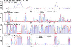
The regime probability diagram of the innovative MSIH (3)-VAR (3) model in Fig. 10 reflects the changing trend and regime probability of China's financial security index (DPAC). Due to the third-order lag of the model, the actual output result is that for May 2004 to June 2018, totaling 171 months. It can be seen from Fig. 10 and Table 13 that China's financial security index (DPAC) has been in the state of Reg. 2 for the longest time, reaching 108 months, accounting for 63.16% of the total sample. This state is a general risk state of financial insecurity (mild), which shows that the stock market bubble index is large and the actual financial security index is unstable, but no serious crisis has broken out yet. April to June 2018, the last sample period of this empirical study, is also in Reg. 2 state, which shows that although China's real economy and capital market encountered certain difficulties in the first half of 2018 with signs of serial default by enterprises, the risk was still controllable.

Fig. 10.

Innovative MSIH (3)-VAR (3) probability map of model area system.

Reg. 1 represents a state of financial insecurity (serious), covering 28 months, accounting for 16.37% of the total sample period; the probability of remaining in Reg. 1 in September-October 2016 and January 2017 is only a little more than 50%, which is not typical. After excluding these three months, the samples of financial insecurity (serious) are 25 months, accounting for 14.62% of the total, which shows that from the whole sample cycle of more than 14 years, there are not many periods when financial security problems were prominent. The financial insecurity (serious) state that can last for several months at a time mainly includes December 2004 to May 2005, August to October 2008, and August 2011 to January 2012. Comparing the common characteristics of these three stages, some basic indexes that constitute the financial security index in this study do not perform well. For example, in 2004 and 2011, the growth rate of fixed assets investment and macroeconomic prosperity index declined due to domestic macro-control. Additionally, in 2008, the GDP growth rate declined due to the subprime mortgage crisis in the United States, and the stock market performed poorly. Thus, these are typical periods of China's financial insecurity (serious).

Reg. 3 implies financial security, low risk, and good financial development, mainly including October 2006 to October 2007, February 2009 to November 2009, and March to June 2015. The common feature of these stages is that the GDP, macro prosperity index, and other indexes performed well, as did the capital market at that time. Thus, moderate prosperity of the capital market helps build up investor confidence and is conducive to national financial security.

The transition probability matrix of the regime in Table 14 lists the transition probability between different regimes. The transition probability between adjacent regimes is higher, while the transition probability between spaced regimes is extremely small.

In the state of regime transformation, the probability of China's financial market remaining in Reg. 1 (transforming to its own regime), that is, maintaining a safe and unsafe (serious) state is 0.565, the probability of transforming from Reg. 1 to Reg. 2 is 0.435, and the probability of directly transforming from Reg. 1 to Reg. 3 is close to 0. This shows that the state of Reg. 1 is unstable, and the probability of switching to other regimes is the highest, which reflects that the probability of the financial market switching from a severe financial insecurity extreme state to a general risk state is very high, and the financial system will not always be in a state of financial crisis. China's financial system is in Reg. 2, that is, the probability of maintaining financial insecurity (mild) is 0.7901, which is much better than that in Reg. 1, indicating that Reg. 2 is relatively stable. The probability of changing from Reg. 2 to Reg. 1 is 0.1272, and the probability of changing to Reg. 3 is 0.08269, that is, the probability of changing to financial security is slightly higher, which also shows that China's financial system as a whole is relatively healthy. The probability of China's financial system remaining in Reg. 3, that is, the financial security state is 0.7827, which is also relatively stable. The probability of changing from Reg. 3 to Reg. 2 is 0.2172. The probability of changing to Reg. 1 is close to 0.

Table 15 presents the count of the probability and duration of maintaining the state of a regime. The probability of China's financial market remaining in the state of Reg. 1 is 0.1749 and the duration is 2.3 months; the probability of Reg. 2 is 0.5977 and the duration is 4.76 months; the probability of Reg. 3 is 0.2274, and the duration is 4.6 months. The data show that China's financial market is in a state of financial insecurity (mild) and financial security for more than 4 months, which is a long time. The duration of financial insecurity (severe) is only half that of other states, and its probability is low. Furthermore, this result is also consistent with the generally held view in finance that financial crises always break out quickly and violently. However, after all parties, especially the regulatory authorities, respond quickly, the crisis can usually be alleviated quickly and effectively.

• (1)

  Correlation statistics under different regimes

As can be seen from Table 16, the correlation coefficient between the stock market bubble index and the financial security index is 0.6657 under Reg. 1, which has a significant positive correlation. This shows that the bigger the stock market bubble index, the bigger the financial security index. Thus, under the condition of financial insecurity (serious), the stock market bubble bursts or is at a low level, which is generally accompanied by a stock market plunge. In this case, the existence of an appropriate stock market bubble is beneficial to the improvement of financial security. The correlation coefficient between the stock market bubble index and the financial security index decreases from −0.1915 to −0.271 under Reg. 2 and 3, and the negative correlation gradually increases, which indicates that an increase in the stock market bubble will bring about a decline in the degree of financial security when the actual financial market security situation is good. This is an interesting result found in this study, as it means that when dealing with the relationship between stock market bubbles and financial security, if the state of financial security is acceptable, the stock market bubble should be properly controlled, and the bubble is the unstable factor of the market at this time. However, when the financial system is in a state of financial insecurity (serious), introducing measures to stimulate the capital market moderately and raising the level of the stock market bubble index moderately may help alleviate financial insecurity.

• (1)

  Impulse response and goodness of fit analysis

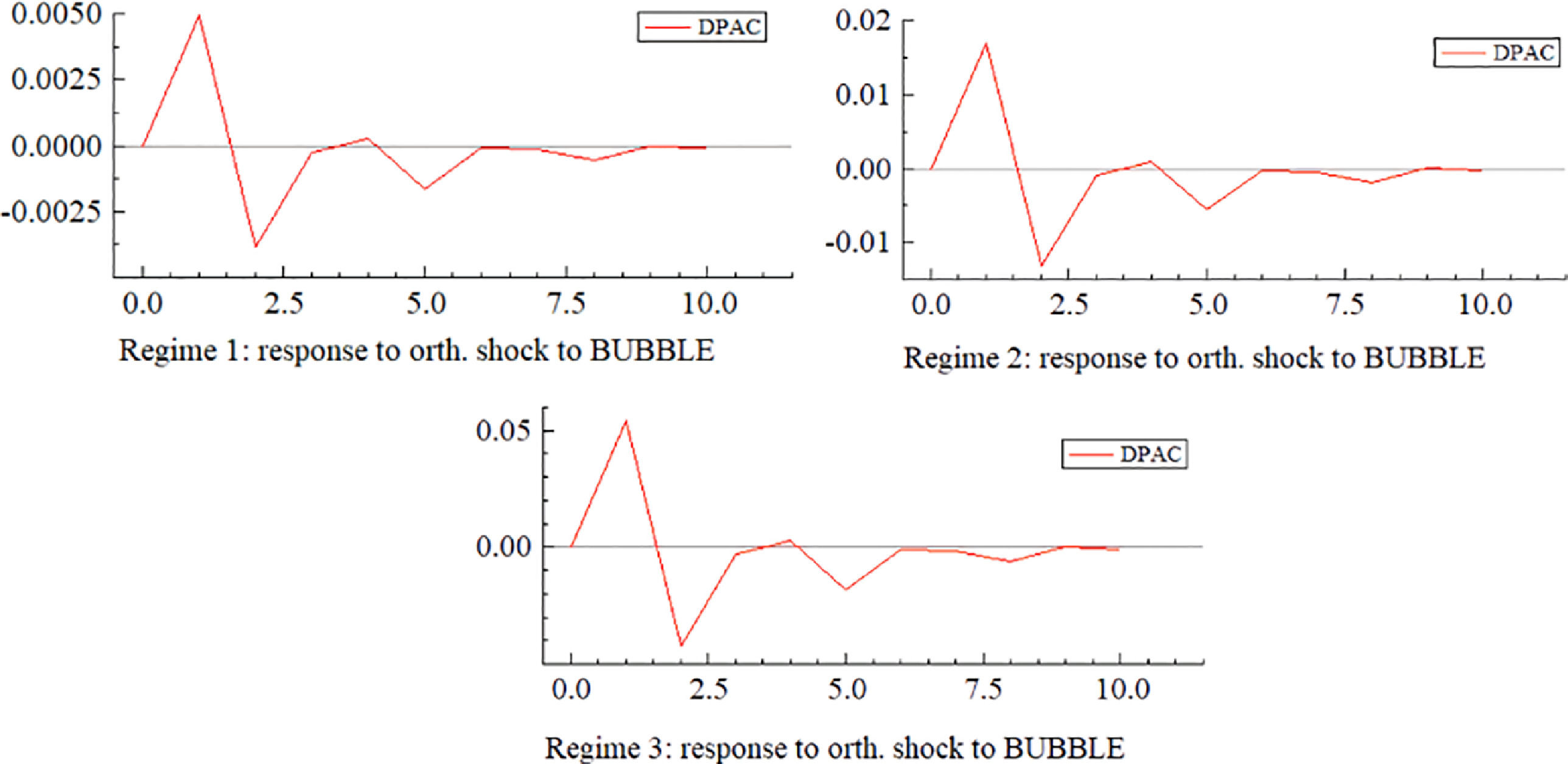
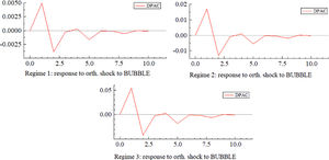
Fig. 11 shows the impulse response of the stock market bubble index to the financial security index (DPAC) under three regimes. First, from the response direction, when the stock market bubble index (BUBBLE) brings a positive impact of one unit, the financial security index responds positively and reaches its peak in the lag of about one period. Then, the index falls rapidly, turns into a negative response, and reaches its lowest point in lag phase 2. Subsequently, the impact strength of each period slowly dips below the abscissa axis, and the fluctuation gradually decreases and reaches a stable state after lag phase 8. Generally speaking, except for the positive response of the first financial security index, the other periods are mainly a negative response, that is, the stock market bubble increases, the degree of financial security rises in the short term, and there is an overall decline.

Fig. 11.

Impulse response diagram under different zone conditions.

Second, from the perspective of response strength, with a decrease in the degree of risk, the impact effect reflected by the impulse response diagram is stronger. Under Reg. 1, the impact of one unit of the stock market bubble index (BUBBLE) on the financial security index reached a peak value of 0.005 in lag phase 1, and then fell to the lowest point of −0.004. However, in the state of Reg. 2, the peak value of the impact force is about 0.017 when in lag phase 1, and the lowest value is close to −0.018 when in lag phase 3. Under the condition of Reg. 3, the peak value of impact force reaches 0.052, and the lowest value reaches about −0. 052; the impact force is the largest and the impact effect is the most obvious. Thus, to improve financial security by regulating the degree of the stock market bubble, we should try our best to plan, and carry out directional regulation in the stages of Reg. 3 and Reg. 2, while in the state of Reg. 1, the policy effect is much worse under the same regulation intensity.

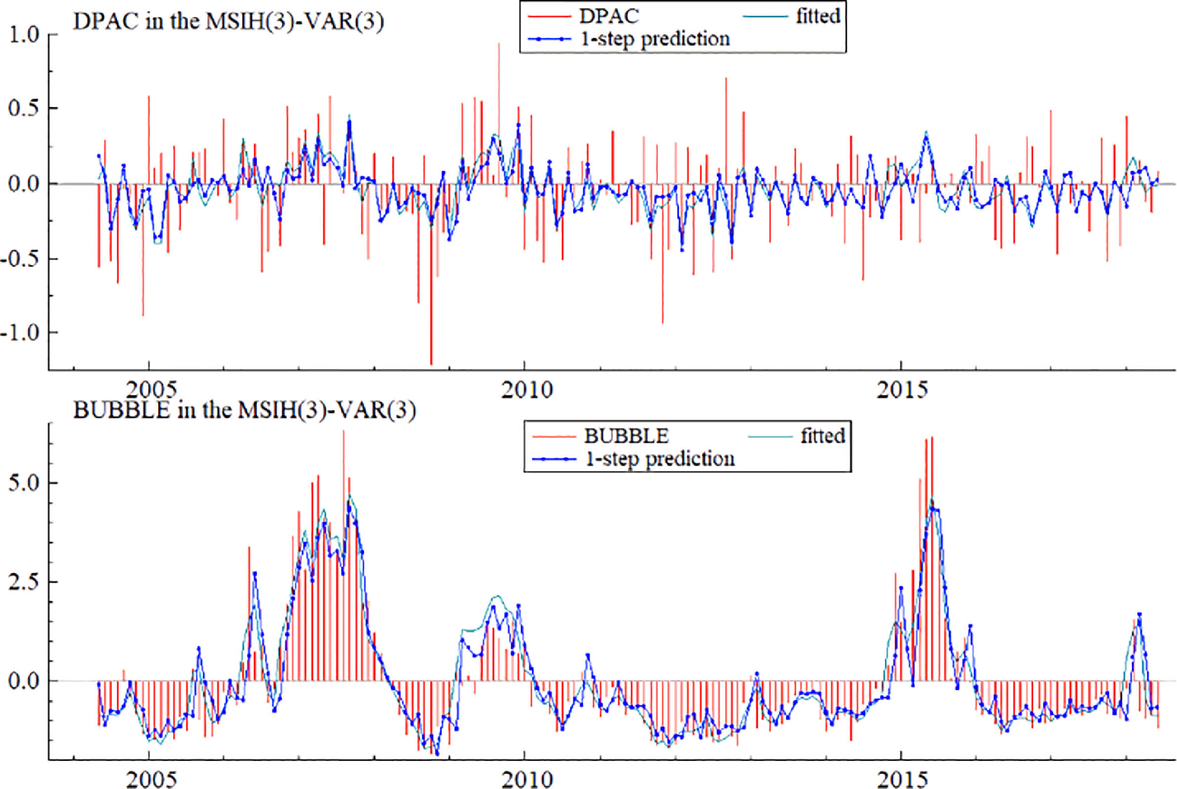
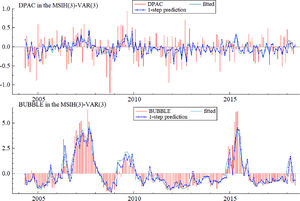
Fig. 12 presents the relationship between the actual values, fitted values, and one-step predicted values of the financial security index (DPAC) and stock market bubble index (BUBBLE) variables. The actual values, fitted values, and predicted values of the stock market bubble index are consistent with each other, and the effect is good; there is a slight error between the actual and predicted values of the financial security index, which may be due to the many influencing factors of the financial security index. However, as the basic movement directions of these variables are consistent, the fitting effect should be acceptable.

Fig. 12.

Actual value, fitted value, and one-step predicted value of the variable. (For interpretation of the references to colour in this figure legend, the reader is referred to the web version of this article.)

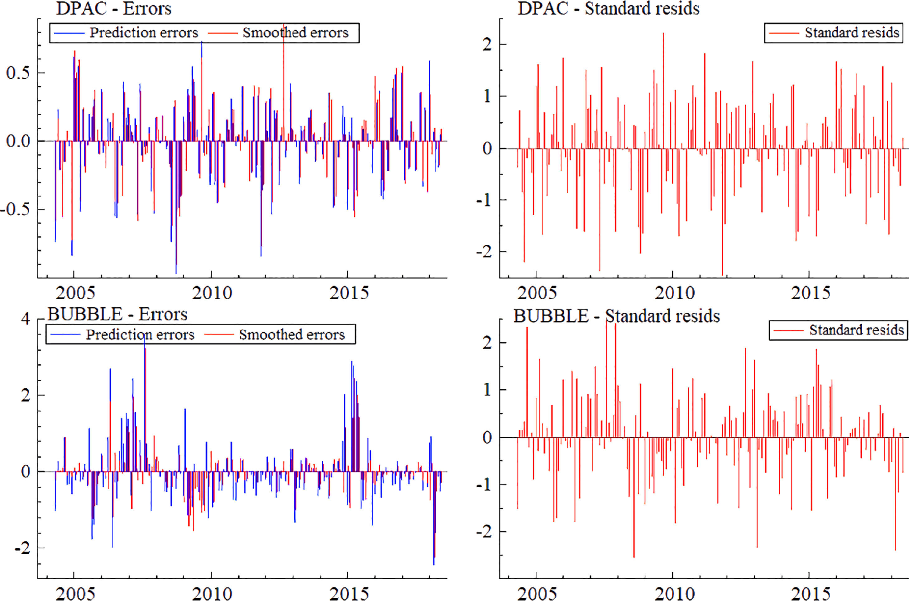
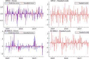
Fig. 13 shows the results of a comparison among variable prediction error, smoothing error, and standard residual. The distribution frequency of prediction error and standard residual is similar. Thus, the innovative MSIH (3)-VAR (3) model has a good fitting effect for each variable, and the results analyzed by the innovative MSIH (3)-VAR (3) model are robust.

• (1)

  Robustness test

Fig. 13.

Prediction error, smoothing error, and standard residual of the variable. (For interpretation of the references to colour in this figure legend, the reader is referred to the web version of this article.)

To verify the robustness of the conclusion of the innovative MSIH (3)-VAR (3) model which contains three regimes and three lag periods, we introduce the multiple linear regression method to study the relationship between the stock market bubble and financial security. As the main research objective of this study is to investigate the impact of the stock market bubble index (BUBBLE) on the financial security index (DPAC), the regression equation is established with the financial security index (DPAC) and the stock market bubble index (BUBBLE) as explanatory variables. As the financial security index and the stock market bubble index are obtained by principal component analysis, the index already contains many factors; thus, no additional control variables are set in the regression equation. Additionally, referring to the results of related studies, if the influence of the bubble sequence with lag phase 3 on the DPAC sequence is not significant, this regression directly takes the bubble sequence with lag phase 1 and lag phase 2 as explanatory variables, and examines the sign, size, and significance level of regression coefficients to verify the robustness of the innovative MS-VAR test. The sample interval is from January 2004 to June 2018, which is the same as that in the previous data.

The regression equation is:

Where α is the cut-off moment of regression, βt−1,βt−2 are the regression coefficients, and εt is the residual. The results are shown in Table 17.

The regression result can be written as:

Analysis of the regression results shows that the results of α are only significant at the 20% level, and its meaning is not obvious. However, the t value of βt−1 reaches 2.75, which is significant at the 1% level, and the regression coefficient is 0.0821329. Compared to the parameter estimation results of the innovative MSIH (3)-VAR (3) model in Table 12, the coefficient of BUBBLE-1 is 0.042371, which is the same sign and significant. It shows that the previous conclusion is relatively stable, that is, a larger stock market bubble with lag phase 1 will help improve the financial security situation. Similarly, the coefficient of βt−2 in Table 17 is-0.0535974, which is significant at the 10% level. The result has the same sign as the coefficient of −0.0469 of BUBBLE-2 in Table 12, and its size is close to that of BUBBLE-2, which expresses the same economic meaning. This shows that the analysis results of the innovative MS-VAR model are relatively robust, and the model can divide data into regimes, and analyze the results more precisely. Hence, the application of this method is appropriate.

Conclusion and implications

Conclusion

In this study, we establish a model covering investor behavior, SPBs, and financial security problems, and verify the interrelationship between the variables. Through simulation and empirical analyses, we obtain the affirmative conclusion that the above logical framework is established. Specifically, the basic conclusions of this study are as follows:

• (1)

  In this study, a comprehensive analysis method is used to superimpose some basic value and investor behavior characteristics, such as irrational investors without financial knowledge, and stock price fluctuation indicators. Subsequently, we extract the principal components, filter out the noise by the Kalman filtering method, and then construct the final SPB index. The SPB index in this study can not only synchronize with the sharp rise and fall of the stock market but also reveal the extent of support of the real economy in the rising stock market, which further confirms that the selected principal component index can better measure the size of the stock market bubble.

• (2)

  The corresponding indicators are selected according to economic security, banking, and insurance security, capital market security, and money market security. Subsequently, China's financial security index is constructed based on the principal component method. The results show that during the sample period, China's financial security index has experienced roughly five fluctuations in the same direction. The performance of the financial security index in each stage is driven by the main economic indicators and has a profound economic background.

• (3)

  In this study, the stock bubble index discussed in Section 4 represents the bubble level, and the financial security index discussed in Section 5 represents the level of China's financial security. The innovative MS-VAR model with a three-zone system and 3 lag stages is established (innovative MSIH (3) -VAR (3)), and the dynamic relationship between them is examined. The results show that the relevant parameters of the model are significant and have obvious economic significance.

First, a Granger causality test is carried out on the stable first-order differential financial security index (DPAC) and stock market bubble index (BUBBLE). The test results show that at the 5% significance level, we accept the original hypothesis that the financial security index is not the cause of the stock market bubble index. There is a unilateral Granger causality relationship between the stock market bubble index and the financial security index, that is, a change in the stock market bubble index can be used to explain changes in the financial security index.

Second, according to the division results of the innovative MSIH (3) – VAR (3) model, Reg. 1–3 represent financial insecurity (serious), financial insecurity (mild), and financial security, respectively. An increase of 1 unit in the stock market bubble index with lag period 1 will lead to an increase in the financial security index of 0.042371 units, while an increase in 1 unit stock of the market bubble index with lag period 2 will reduce the financial security index by 0.0469 units. This shows that the stock market bubble index is the leading indicator of financial security.

Third, from the analysis of the results of the three-regime innovative MSIH (3) - VAR (3) model, the probability of China's financial security status staying in Reg. 2 and Reg. 3 is large, and the duration of Reg. 1 is only about half of that of the other regimes. This shows that China's financial security situation is relatively stable and is in a relatively safe financial state most of the time, and the possibility of systemic financial risk is small.

Fourth, from the perspective of correlation, the stock market bubble index is positively related to the financial security index under Reg. 1, and the correlation is negative under the other two regimes. The conclusion has significant implications for policymakers because Reg. 1 is a state of few stock market bubbles and financial insecurity (severe). It shows that when the financial situation is seriously unsafe, and stock market bubbles are few, policymakers can take measures to increase positive interest in the securities market and stimulate activity, that is, expand the stock market bubble to improve the security situation of the financial market.

Fifth, the impulse response results show that given the positive impact of a unit stock on the market bubble index, the financial security index reaches a positive response peak in lag period 1, turning to a negative response and reaching the lowest point in lag period 2. Thereafter, the fluctuation slows down and reaches a stable state after lag period 8. This also shows that the initial impact of the stock market bubble on the financial security situation is a positive driving force, which will then turn negative and lead to a reduction in the degree of financial security.

The above empirical conclusions can help us further understand the intrinsic relationship between China's stock market bubble level and financial security level, to facilitate regulators to introduce more targeted regulatory measures to respond to market concerns and to monitor market pain.

Implications

First, investors should strengthen the study of financial knowledge. Investors should study investment books, attend financial education lectures, and opt for higher education and other ways to learn relevant financial knowledge, improve their analysis and judgment ability, and try to form a stable investment method system based on their own characteristics.

Second, investors should learn to control their emotions. Investors should be clear about the importance of controlling emotions so that they can make the most favorable judgment when their emotions fluctuate. In the face of a complex and changeable stock market environment, investors should have the ability to think independently, exercise rational investment thinking, and avoid wrong practices such as "chasing up and killing down", "psychological account", and "herding effect".

Thirdly, investors should strengthen the ability of information collection and judgment. Due to information asymmetry and other characteristics of the stock market, the investment judgment formed by investors, based on diverse information, is often very different. Therefore, when investors pay attention to real-time dynamic information about the market, they should not only avoid blind listening and obedience, but should also not be over-confident, and should grasp the appropriate scale.

This study used the basic value method, GSADF method, and other methods to empirically test the bubble level of China's securities market, and compare the results of different methods. It is found that Tobin's Q method and K bubble coefficient method are too simplistic, and may leave out important information, thus presenting the wrong bubble index. The GSADF method finds out whether there is a bubble from the stock price itself, and does not relate to the basic value. Moreover, its recursive algorithm may also lead to insensitivity to the partial fluctuations in the share price. After repeated comparisons and attempts, we choose to use a series of indicators including basic value, investor behavior indicators, and stock price fluctuation indicators to construct the SPB index. The result is consistent with the actual market trend, and the measurement of the bubble level is better than with other methods.

In the study of stock market bubbles affecting financial security, the general view is that stock market bubbles are not conducive to financial security. However, no study in the literature has discussed the micro-mechanism and time lag effect of the stock market bubble affecting financial security. The positive effects of stock bubbles with lag phase 1 on financial security and the negative effect of the stock market bubble with lag phase 2 on financial security are found in this study, which provides new perspectives and evidence for the research in this field.

However, this study has some limitations. The coverage of this index is not extensive enough to ensure the causality of the bubble index and safety index, as the design methods of stock market bubbles and financial safety monitoring indicators are not sophisticated enough.

Based on the above research methods and conclusions, the following are possible further research directions: First, we should enrich and improve the index design based on integrated basic values and emotions, and further analyze the critical level of bubble rupture, to provide early warnings for market participants and provide timely and accurate suggestions for regulatory authorities to deal with market risks; second, we can study the internal structure and interaction mechanism of stock index bubbles, such as industry and scale, and analyze the bubble situation of each sub-industry, and their interaction with each other and the overall bubble situation; finally, the research on stock market bubbles can be expanded to the study of asset bubbles including real estate bubbles, the existence and interaction mechanism of stock market and housing bubbles, and the impact of asset price bubbles on financial security.)

Table 2.

Results of principal component analysis.

Eigenvalues: (sum= 5, mean= 1)
Number	Value	Difference	Proportion	Cumulative Value	Cumulative Proportion
1	2.988553	1.699787	0.5977	2.988553	0.5977
2	1.288766	0.794237	0.2578	4.277319	0.8555
3	0.494529	0.341064	0.0989	4.771848	0.9544
4	0.153465	0.078778	0.0307	4.925313	0.9851
5	0.074687	—	0.0149	5	1

Table 3.

Alternative indicators of financial security index construction.

First-level Index	Second-level Index	Third-level Index
Macroeconomic System	Economic Operation	GDP growth rate, Fixed-asset investment growth rate of the whole society, Macroeconomic prosperity leading index
	Financial Policy	The year-on-year growth rate of M2
Banking and Insurance System	Banking System	Non-performing loan ratio of commercial banks, Monthly standard deviation of interbank 7-day lending rate
	Insurance System	The growth rate of insurance assets, the Growth rate of insurance total compensation
Capital Market System	Stock Market	Monthly standard deviation of the exchange rate between the US dollar and RMB, Monthly standard deviation of the Shanghai Composite Index
Monetary System	Internal Value	CPI
	External Value	Monthly standard deviation of the exchange rate between the US dollar and RMB

Note: the volatility index of the real effective exchange rate is replaced by the monthly standard deviation of the exchange rate between the US dollar and the RMB.

Table 4.

Principal component eigenvalue and variance contribution rate.

Principal component	Characteristic value	Difference in characteristic value	Variance contribution rate	Cumulative variance contribution rate
1	3.601866	1.960044	0.3274	0.3274
2	1.641822	0.162503	0.1493	0.4767
3	1.479318	0.373822	0.1345	0.6112
4	1.105496	0.235332	0.1005	0.7117
5	0.870164	0.104335	0.0791	0.7908
6	0.765829	0.224963	0.0696	0.8604
7	0.540866	0.057567	0.0492	0.9096
8	0.483299	0.133883	0.0439	0.9535
9	0.349417	0.249748	0.0318	0.9853
10	0.099668	0.037414	0.0091	0.9943
11	0.062254	—	0.0057	1

Table 5.

KMO and SMC values of variables.

Variable	KMO Value	SMC Value
Xu1_ s	0. 7112	0. 9764
x2_ s	0. 6546	0. 7213
x3_ s	0. 7643	0. 9101
x4_ s	0. 6337	0. 7121
x5_ s	0. 6587	0. 5915
x6_ s	0. 5833	0. 8432
x7_ s	0. 6443	0. 8399
x8_ s	0. 7768	0. 9324
Total	0. 7051	——

Table 6.

Factor load matrix.

	principal component 1	principal component 2	principal component 3	principal component 4	principal component 5
CPI: YoY of the current month	0.790907	0.048536	0.021245	−0.10428	0.102275
Fixed asset investment: YoY in the current month	−0.212755	0.675686	0.057535	0.466233	0.02256
M2: YoY	0.101815	0.991439	−0.004706	0.027704	−0.076769
Insurance companies: growth rate of total assets	−0.039419	0.120281	−0.155508	0.164406	0.020135
Insurance companies: growth rate of cumulative compensation value	−0.006432	0.016447	−0.414305	0.08599	−0.149453
GDP: quarter on quarter	−0.522718	0.588089	0.017694	0.403825	−0.033709
Proportion of non-performing loans: Commercial Banks	0.120996	−0.161736	−0.028825	−0.977665	−0.050419
Monthly standard deviation of the central parity of US dollar against RMB	0.017289	0.014753	0.998969	0.038951	0.00524
Monthly standard deviation of 7-day weighted interest rate of interbank lending	0.566079	0.16158	0.088405	0.0059	0.043038
Monthly standard deviation of Shanghai Composite Index	0.04607	−0.055189	0.013232	0.045573	0.996283
Macroeconomic prosperity index: leading index	−0.672656	0.675787	0.006956	0.300185	0.026202

Table 7.

Matrix of factor scores coefficients.

	principal component 1	principal component 2	principal component 3	principal component 4	principal component 5
CPI: YoY of the current month	4.44E-16	−2.50E-16	−6.94E-17	−3.33E-16	0
Fixed asset investment: year on year in the current month	2.22E-16	−4.44E-16	0	−4.44E-16	5.55E-17
M2: YoY	0.904338	0.917608	−0.027716	−0.03964	0.011194
Insurance companies: growth rate of total assets	9.71E-17	1.94E-16	−2.78E-17	0	−3.47E-18
Insurance companies: growth rate of cumulative compensation value	−2.78E-17	−2.78E-17	0	−2.78E-17	5.55E-17
GDP: quarter on quarter	0	−1.33E-15	−2.78E-17	−8.88E-16	5.55E-17
Proportion of non-performing loans: Commercial Banks	−0.405285	0.077936	0.048025	−1.091042	0.072328
Monthly standard deviation of the central parity of US dollar against RMB	0.001286	0.004539	1.002156	−0.029532	−0.011767
Monthly standard deviation of 7-day weighted interest rate of interbank lending	−3.33E-16	−2.22E-16	−5.38E-17	−1.67E-16	−2.78E-17
Monthly standard deviation of Shanghai Composite Index	0.086427	0.070475	−0.00576	−0.052679	1.006125
Macroeconomic prosperity index: leading index	−1.416709	0.157854	0.029807	−0.206621	0.083312

Table 8.

Unit root test results.

Variable	ADF test value	Critical value (1%, 5%, 10%)			Stationary conclusion
PAC	−1.889916	−3.46898	−2.878413	−2.575844	Unstable
DPAC	−5.54117	−3.46898	−2.878413	−2.575844	stable
BUBBLE	−3.462728	−3.468295	−2.878113	−2.575684	stable

Table 9.

Granger causality test.

Original hypothesis	F-Statistic	Probability
DPAC is not Granger of bubble	0.75562	0.5206
Bubble is not Granger of DPAC	3.22792	0.024

Table 10.

The lag order under each criterion.

Lag	Log L	LR	FPE	AIC	SC	HQ
0	−386.144	NA	0.348195	4.620762	4.657952	4.635856
1	−262.8288	242.2263	0.084129	3.200343	3.311914*	3.245624*
2	−261.0552	3.441712	0.086391	3.226848	3.412798	3.302315
3	−253.811	13.88470*	0.083123*	3.188226*	3.448557	3.293881
4	−252.9926	1.549108	0.086341	3.226103	3.560813	3.361944

Table 11.

Innovative MS-VAR model selection.

	linear system	nonlinear system
	VAR(3)	MSM(3) VAR(3)	MSMH(3) VAR(3)	MSI(3) VAR(3)	MSIH(3)-VAR(3)	MSIAH(3)-VAR(3)
LL	−249.3532	−242.6538	−203.144	−214.977	−189.2759	−173.97
AIC	3.19216	3.1724	2.7782	2.8468	2.615*	2.7173
HQ	3.455695	3.3745	3.0252	3.0489	2.862*	3.1439
SC	3.299138	3.6704	3.3869	3.3448	3.2237*	3.7687

Table 12.

Innovative MSIH (3)-VAR (3) parameter estimation results of the model.

	DPAC EQUATION		BUBBLE EQUATION
	COEFFICIENT	T VALUE	COEFFICIENT	T VALUE
INTERCEPT(Reg.1)	−0.177813	−1.7821*	−0.703765	−12.9494***
INTERCEPT(Reg.2)	−0.062921	−2.0474**	−0.281587	−4.7875***
INTERCEPT(Reg.3)	0.168304	3.1125***	1.311652	3.7318***
DPAC_1	−0.175945	−2.5762***	0.139927	2.2278**
DPAC_2	0.056903	0.8703	−0.012125	−0.1702
DPAC_3	0.293276	4.4823***	0.171992	2.2928**
BUBBLE_1	0.042371	1.5006*	0.506697	8.6555***
BUBBLE_2	−0.0469	−1.3903*	0.07047	1.2881*
BUBBLE_3	−0.000684	−0.0249	−0.029176	−0.748
Standard Error (Reg.1)	0.468971		0.156089
Standard Error (Reg.2)	0.250547		0.4083
Standard Error (Reg.3)	0.263038		1.328542

Note: *, **, *** are significant at 10%, 5% and 1%, respectively.

Table 13.

Innovative MSIH (3)-VAR (3) regime sampling time and probability of the model.

Reg.1	Time interval	Probability	Reg.2	Time interval	Probability
	2004:5 - 2004:5	[0.9876]		2004:6 - 2004:11	[0.9208]
	2004:12 - 2005:5	[0.8698]		2005:6 - 2005:7	[0.9613]
	2006:8 - 2006:8	[0.8377]		2005:9 - 2006:3	[0.8890]
	2008:8 - 2008:10	[0.9725]		2006:6 - 2006:7	[0.8507]
	2011:8 - 2012:1	[0.8143]		2006:9 - 2006:9	[0.9810]
	2012:3 - 2012:4	[0.7701]		2007:11 - 2008:7	[0.9069]
	2012:7 - 2012:10	[0.8593]		2008:11 - 2009:1	[0.9459]
	2016:4 - 2016:5	[0.9111]		2009:12 - 2011:7	[0.8755]
	2016:9 - 2016:10	[0.5268]		2012:2 - 2012:2	[0.9994]
	2017:1 - 2017:1	[0.5746]		2012:5 - 2012:6	[0.9189]
REG.3	Time interval	Probability		2012:11 −2014:10	[0.9028]
	2005:8 - 2005:8	[0.6945]		2015:1 - 2015:2	[0.8311]
	2006:4 - 2006:5	[0.9589]		2015:7 - 2016:3	[0.7326]
	2006:10 −2007:10	[0.9973]		2016:6 - 2016:8	[0.9879]
	2009:2 - 2009:11	[0.9579]		2016:11 −2016:12	[0.7511]
	2014:11 −2014:12	[0.9619]		2017:2 - 2017:12	[0.9582]
	2015:3 - 2015:6	[1.0000]		2018:4 - 2018:6	[0.8579]
	2018:1 - 2018:3	[0.8737]

Table 14.

Regime switching probability matrix.

	Reg. 1	Reg. 2	Reg. 3
Reg. 1	0.565	0.435	6.10E-07
Reg. 2	0.1272	0.7901	0.08269
Reg. 3	0.0001374	0.2172	0.7827

Table 15.

Regime status and duration.

	Sample size	Probability	Duration
Reg. 1	30.5	0.1749	2.3
Reg. 2	101.2	0.5977	4.76
Reg. 3	38.3	0.2274	4.6

Table 16.

Correlation statistics under different regimes.

Reg. 1	DPAC	BUBBLE
DPAC	1	0.6657
BUBBLE	0.6657	1
Reg. 2	DPAC	BUBBLE
DPAC	1	−0.1915
BUBBLE	−0.1915	1
Reg. 3	DPAC	BUBBLE
DPAC	1	−0.271
BUBBLE	−0.271	1

Table 17.

Multivariate regression results.

DPAC	coef	std.err	t-value	P>|t|
Bubble(t-1)	0.0821329	0.0298472	2.75***	0.007
Bubble(t-2)	−0.0535974	0.0298655	−1.79*	0.075
_cons	−0.0369546	0.0258777	−1.43	0.155

Note: *, **, *** are significant at 10%, 5% and 1%, respectively.

Abbreviations and acronyms

AIC	Akaike information criterion
BUBBLE	Stock market bubble index
CPI	Consumer price index
DPAC	First-order differential financial security index
FPE	Final prediction error
GDP	Gross domestic product
HQ	Hannan-Quinn criterion
KMO	Kaiser-Meyer-Olkin
LL	Logarithmic likelihood
LR	Likelihood ratio
M	Number of shares traded
M2	Broad money supply
N	Total stock market capitalization on SSE
PAC	Financial security index
P/E	Price to earnings ratio
R	Stock turnover amount
Reg.	Regime
S	Comprehensive evaluation score for each year
SC	Schwarz criterion
SMC	Squared multiple correlations of variables with all other variables
SPB	Stock price bubble
SPBF	SPB index by applying the Kalman filter algorithm
SSE	Shanghai Stock Exchange
TTR	Total market capitalization-weighted monthly market turnover ratio