To support the assessment of R&D project portfolios and to establish a systemic model to carry multiple evaluations using the decision-maker knowledge, preferences and purposes we have developed an evaluation matrix and a new procedure based on the PROV exponential decision method which uses multiple utility functions modeled to establish a common framework from which we can determine the projects relative value. The presentation of this new procedure is the main focus of this article and numerical examples are presented to illustrate the proposed approaches to attain comprehensible results and to discover the most valuable R&D projects to support investment decisions.
Research and development (R&D) is the predecessor of new knowledge, patents and technology which might be converted into new innovations, enhanced products or explicit or tacit knowledge. To select and prioritize the most promising R&D projects multicriteria evaluation methods can be employed to capture the value of far-reaching opportunities under high uncertainty. R&D investment decisions are usually taken based on data which is highly uncertain and often very inaccurate, with very unclear technical applications, life time expenditure and market outcomes (Eldermann, 2012). To prevail over and to overcome some degrees of uncertainty and risk inherent to R&D projects, we aggregated in an evaluation matrix, some of the main criteria used to prioritize R&D projects, and we proposed a new multicriteria procedure to create a predefined model to assess multiple projects considering the decision-maker knowledge, preferences and purposes. Among the most known multicriteria decision methods addressing the decision-maker preferences and objectives are the AHP, Analytic Hierarchy Process (Canada & Sullivan, 1989; Munier, 2011; Saaty, 1980, 2005), the ELECTRE, Élimination et Choice Traduisant la Réalité (Figueira & Roy, 2005; Rogers, 2001; Munier, 2011) and the PROMETHEE, Preference ranking organization method for enrichment evaluations (Brans & Mareschal, 2005; Munier, 2011). Foreseeing a convergent goal, we have other methods, such as the PROV Exponential Decision Method (Rocha, Tereso, & Ferreira, 2012). The proposed procedure to create a predefined model to assess multiple projects is based on this last method. The assessment matrix and the new procedure based on the PROV Exponential decision method are described in the following sections, where we define their scope and purpose and where we present its application procedure.
2Evaluation matrix to assess R&D projectsThe evaluation matrix to assess R&D projects was developed to assess far-reaching ideas and to capture the value of future opportunities under high uncertainty. This matrix converts available and prospective information on quantifiable criteria organized in aggregation groups with different relative weights purposefully defined to include tangible and intangible assets.
Knowledge intensive organizations usually have a portfolio of pending ideas and projects to which they can recur to develop current products or to seize new inventions, technologies or products. These portfolios can also be referred as the organizations strategic options (Eldermann, 2012).
Strategic options, like R&D project proposals, can be difficult to assess due to the uncertain future of their results and there may be no clear understanding of their innovations prospective market potential. Knowing the difficulty of assessing far-reaching ideas, evaluation methods can be better used by reviewing the organizations current resources, networks and purposes, making them present as a part of the evaluation method.
The evaluation matrix is structured in seven aggregation groups including dimensions linked to the organization resources, networks and business strategy.
A – Advancement status and engaged resources: the existence of previous R&D results supporting the need for further research, and the available infrastructures and human resources with the abilities and engagement required for the project development;
B – R&D final applications differentiation: the uniqueness of the technology pursued and their manufacturing potential and ease-of-use;
C – Applications relevance and time-to-market: the project prospective resulting applications and their relevance for the institution operational and expansion activities, and perceived or expected expressions of interest and time needed to display a marketable technology;
D – Competing research projects: the existence of concurrent R&D teams and their ability to raise resources;
E – Competing applications: the available alternatives of solution (if available) pursuing similar purposes;
F – Investment and operational costs of the R&D project: the required investment and operational additional costs with the R&D project after discounting public funds (if available);
G – Profitability: the prospective applications pursued by the R&D project net-present value, internal rate of return and pay-back-period.
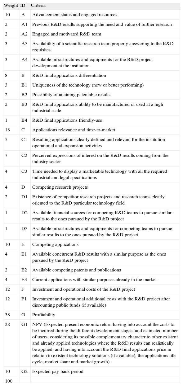
In Table 1 is presented the aggregation groups and their relative criteria, established by reviewing the works of Eldermann (2012), Razgaities (2003) and Speser (2006), and their proposed measuring scales are presented in appendix. A weights proposal is also suggested, just for the purpose of supporting the presentation of a numerical example, described on the third section of this article.
Evaluation matrix for strategic R&D projects assessment.
| Weight | ID | Criteria |
| 10 | A | Advancement status and engaged resources |
| 2 | A1 | Previous R&D results supporting the need and value of further research |
| 2 | A2 | Engaged and motivated R&D team |
| 3 | A3 | Availability of a scientific research team properly answering to the R&D requisites |
| 3 | A4 | Available infrastructures and equipments for the R&D project development at the institution |
| 8 | B | R&D final applications differentiation |
| 3 | B1 | Uniqueness of the technology (new or better performing) |
| 2 | B2 | Possibility of attaining patentable results |
| 2 | B3 | R&D final applications ability to be manufactured or used at a high industrial scale |
| 1 | B4 | R&D final applications friendly-use |
| 18 | C | Applications relevance and time-to-market |
| 7 | C1 | Resulting applications clearly defined and relevant for the institution operational and expansion activities |
| 7 | C2 | Perceived expressions of interest on the R&D results coming from the industry sector |
| 4 | C3 | Time needed to display a marketable technology with all the required industrial and legal specifications |
| 4 | D | Competing research projects |
| 2 | D1 | Existence of competitor research projects and research teams clearly oriented to the R&D particular technology field |
| 1 | D2 | Available financial sources for competing R&D teams to pursue similar results to the ones pursued by the R&D project |
| 1 | D3 | Available infrastructures and equipments for competing teams to pursue similar results to the ones pursued by the R&D project |
| 10 | E | Competing applications |
| 4 | E1 | Available concurrent R&D results with a similar purpose as the ones pursued by the R&D project |
| 2 | E2 | Available competing patents and publications |
| 4 | E3 | Current applications with similar purposes already in the market |
| 12 | F | Investment and operational costs of the R&D project |
| 12 | F1 | Investment and operational additional costs with the R&D project after discounting public funds (if available) |
| 38 | G | Profitability |
| 28 | G1 | NPV (Expected present economic return having into account the costs to be incurred during the different development stages, and estimated number of users, considering its possible complementary character to other existent and already applied technologies where the R&D results can realistically be applied, and having into account the R&D final applications price in relation to existent technology solutions (if available), the applications life cycle, market share and market growth). |
| 10 | G2 | Expected pay-back period |
| 100 |
The criteria weights can be assigned directly to every criterion or a formal method can be used, such as the AHP weighing procedure (Saaty, 2005; Hobbs & Meier, 2003) where the weights are attained by establishing paired-wise comparisons.
3Application procedureThe PROV Exponential Decision Method (Rocha et al., 2012) was developed to express the stakeholders knowledge, objectives and preferences to attain comprehensible results and to discover the most adequate solution for a problem or to accomplish a certain goal and the ordering and relative value of the alternative solutions (our options).
Through the modelation of the stakeholders thoughts and purposes this method allows to develop an informed evaluation having in mind all the options which are visually shown on a graphical representation. This graphical representation presents the options relative position on two lines, one expressing a linear growth which means that increments of the same size have equal importance, and another line expressing the real value attributed by the decision-maker having into account that as some milestones are attained, the importance attributed to greater values may decrease, since some value of satisfaction has been attained. It also allows the decision maker to express the interval of values at which he considers the options indifferent among each other. He can also express that the options in a determined interval of values have a closer importance and as they get away from this interval the value of those options decrease intensively. The decision-maker can also express the decrease of preference if, at a determined level the continuous growth becomes nefarious for the problem under analysis.
This method has been presented, by the authors of this article, on the Proceedings of the World Congress on Engineering 2012, on this current work, we’re just going to present some of its steps and the concepts of nefarious values won’t be addressed, since their content and features aren’t required for projects portfolio assessment.
On the following description, we’re also going to add new insights into the method on how to establish a common reference scale to assess the value of multiple projects by introducing new data into a predefined evaluation matrix. This procedure is going to be presented using the previously proposed evaluation matrix, and its application can be understood by following the subsequent steps. For the purpose of illustration, numerical examples will be used:
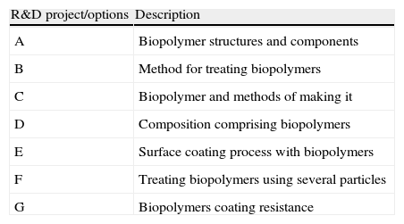
1st Identify the R&D projects, also referred as options, to be evaluated (for this purpose, we used seven hypothetical projects, represented by the letters A to G, within a research area, see Table 2);
R&D projects identification.
| R&D project/options | Description |
| A | Biopolymer structures and components |
| B | Method for treating biopolymers |
| C | Biopolymer and methods of making it |
| D | Composition comprising biopolymers |
| E | Surface coating process with biopolymers |
| F | Treating biopolymers using several particles |
| G | Biopolymers coating resistance |
2nd Review the R&D projects assessment matrix to check if all the relevant criteria, for the purpose of our analysis, are contemplated and make any change in accordance to that purpose;
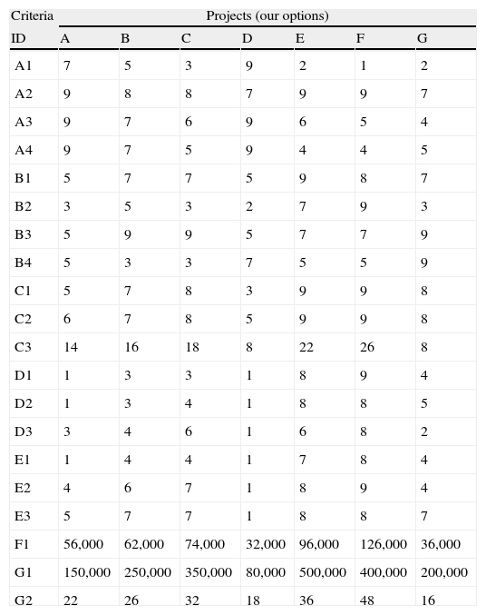
3rd Identify the attributes for each project, by referring to the criteria measuring scales, presented in appendix, or to any other scale considered relevant and establish a matrix with those attributes, see Table 3;
Criteria attributes of every project.
| Criteria | Projects (our options) | ||||||
| ID | A | B | C | D | E | F | G |
| A1 | 7 | 5 | 3 | 9 | 2 | 1 | 2 |
| A2 | 9 | 8 | 8 | 7 | 9 | 9 | 7 |
| A3 | 9 | 7 | 6 | 9 | 6 | 5 | 4 |
| A4 | 9 | 7 | 5 | 9 | 4 | 4 | 5 |
| B1 | 5 | 7 | 7 | 5 | 9 | 8 | 7 |
| B2 | 3 | 5 | 3 | 2 | 7 | 9 | 3 |
| B3 | 5 | 9 | 9 | 5 | 7 | 7 | 9 |
| B4 | 5 | 3 | 3 | 7 | 5 | 5 | 9 |
| C1 | 5 | 7 | 8 | 3 | 9 | 9 | 8 |
| C2 | 6 | 7 | 8 | 5 | 9 | 9 | 8 |
| C3 | 14 | 16 | 18 | 8 | 22 | 26 | 8 |
| D1 | 1 | 3 | 3 | 1 | 8 | 9 | 4 |
| D2 | 1 | 3 | 4 | 1 | 8 | 8 | 5 |
| D3 | 3 | 4 | 6 | 1 | 6 | 8 | 2 |
| E1 | 1 | 4 | 4 | 1 | 7 | 8 | 4 |
| E2 | 4 | 6 | 7 | 1 | 8 | 9 | 4 |
| E3 | 5 | 7 | 7 | 1 | 8 | 8 | 7 |
| F1 | 56,000 | 62,000 | 74,000 | 32,000 | 96,000 | 126,000 | 36,000 |
| G1 | 150,000 | 250,000 | 350,000 | 80,000 | 500,000 | 400,000 | 200,000 |
| G2 | 22 | 26 | 32 | 18 | 36 | 48 | 16 |
4th Analyze the attributes, to verify if the lowest performance of some project, in fundamentally important criteria, makes them unacceptable (this should be done if we have crucial criteria demanding minimum standards to avoid possible compensation by other criteria; the projects below the minimum standards shouldn’t be considered);
5th Determine or assign weights to the criteria. The weights can be assigned directly by the decision-maker or they can be attained using criteria weighting methods. In this case, we’re going to use the weights proposed in Table 1;
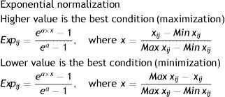
6th Determine the criteria to be maximized (the higher values are the best condition) and to be minimized (the lower values are the best condition) and apply the exponential normalization to the attributes of the measuring scales of every criterion, presented in appendix (if for some of the criteria any measuring scale has been defined, we should establish an utility function from 1 to n or an utility function defined by a sequence of intervals as presented in Tables 10 and 9).
The exponential normalization can be applied according to the following formula (1), where x corresponds to a linear transformation procedure and a corresponds to an independent factor expressing the decision-maker knowledge, preferences and purposes. Afterwards, draw a graph containing two lines (the linear normalization line and the exponential normalization line).
x – corresponds to a linear transformation procedure
a – corresponds to an independent factor
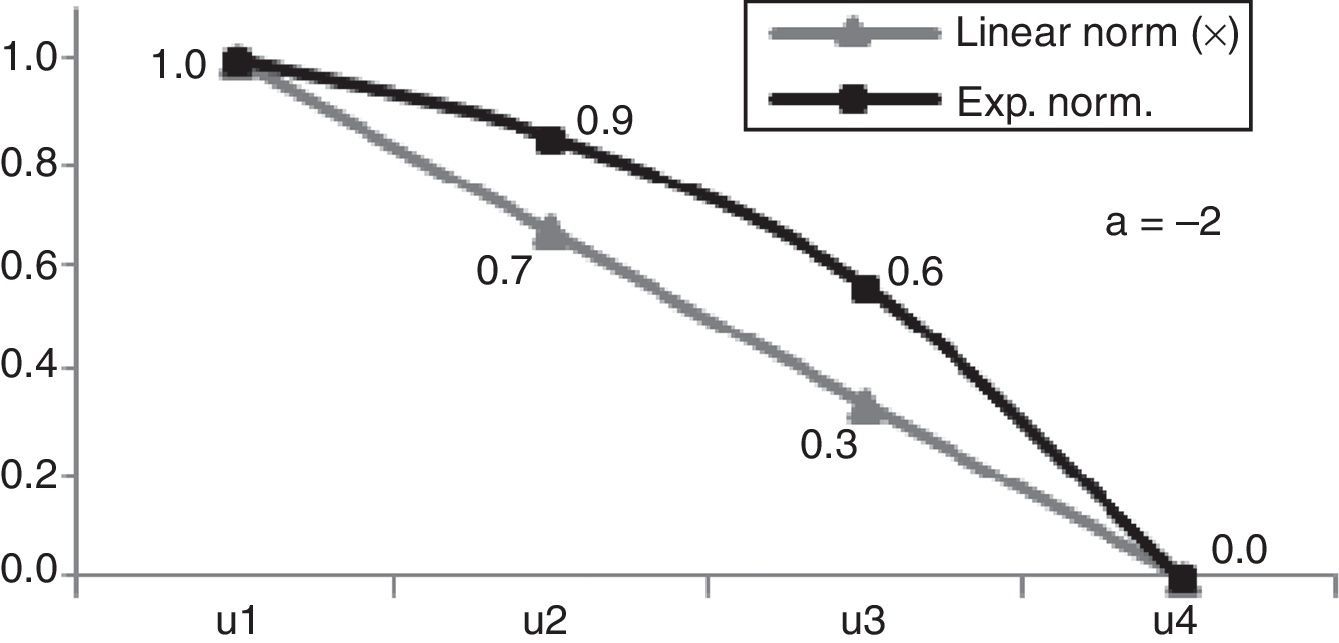
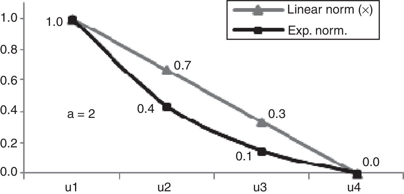
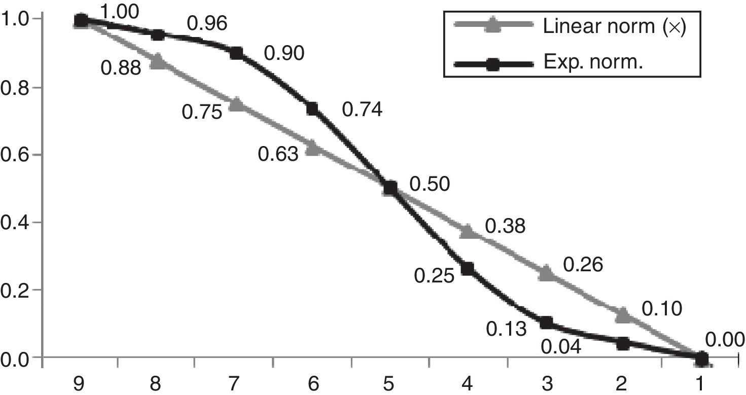
A negative factor a results in a concave exponential growth (Fig. 1). A positive factor a results in a convex one (Fig. 2).
A negative factor a brings closer the best attributes of the utility function and detaches them from the less performing ones. By making factor a more negative those differences become even more significant. A positive factor a brings the decision-maker closer to the best utility function detaching it from all the others increasing the proximity between the less performing utility functions. By making factor a more positive the proximity between the less performing attributes of the utility function is augmented. Therefore, it is possible to adequate the values according to the decision-maker perceptions by changing factor a (Matos, 2005); we can also have more than one factor a.
7th Analyze the lines progression and change factor a to reflect the decision-maker knowledge, preferences and objectives. The decision-maker should take into account the attributes linear progression of the utility function and the reference scale between 0 and 1. This reference scale should be taken as a measure of importance or concordance to translate the decision-maker thoughts and intentions. The attributes of the utility function are more important as they approach 1 and decrease their importance as they decrease till 0. The graph offers a good visual representation of the attributes relative value and we can make judgments having in mind all the attributes under evaluation. In this way, we’re not only making paired-wise comparisons, we’re also performing an integrated assessment of all the attributes of the utility function since we can observe the relative position of all of them in the linear and on the exponential line.
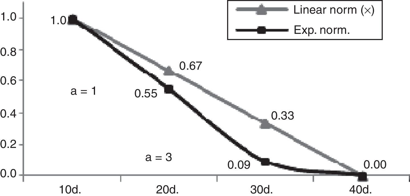
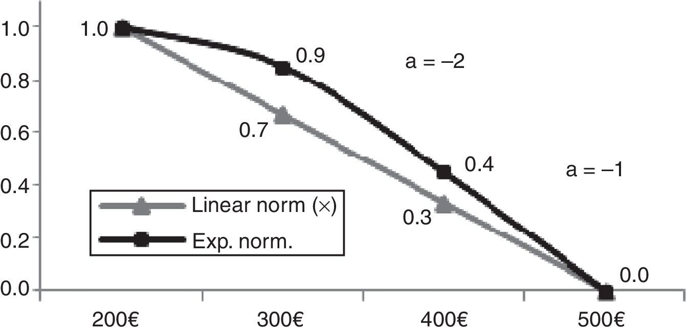
In Figs. 3 and 4 we can observe how factor a supports the modeling of the decision-maker thoughts and intentions by assigning more than one factor a to bring the attributes closer or detached from each other. In Fig. 3 we have two factors a (1 and 3). The first expresses a decrease of value stronger than a linear evaluation would suggest, but as the attributes get lower performances the detachment from the linear normalization line is even greater. This happens because we have a factor a with a value of 3 expressing a significant decrease of value of projects with a 30 days duration bringing them closer to the value of projects with 40 days, which is the longest implementation time. In Fig. 4 we can notice that the decision-maker does not make a significant distinction between the cost of projects between 200€ and 300€, since we have a negative factor a bringing closer these projects. As the cost increases, the decision-maker changes the negative factor a from −2 to −1 meaning that he still considers the projects value a bit greater than the one assigned by a linear value line, detaching it from the most expensive projects.
We can also express graphically, indifference and nefarious threshold (nefarious threshold won’t be presented since they are not required for project portfolios assessment). The indifference threshold refers to a value over which the decision-maker doesn’t make any distinction between the attributes of the utility function on a certain criterion and its establishment is important to avoid conditioning the projects final evaluation result. This threshold can be graphically modeled by assigning a positive or negative factor a till a level at which the attributes become indifferent (with the same value) among themselves. If all attributes have exactly the same importance, we don’t need to model graphically the utility function of one criterion, and we should assign to all of them the same attribute. In this case, the relative value of the projects is given by a linear normalization procedure.
8th Determine the projects relative value on every criterion following a four stages procedure:
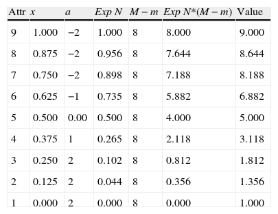
1st stage: Multiply the exponential normalization results by the difference between the criterion maximum and minimum value (see Table 4);
Utility function for the attributes of criterion B2 – possibility of attaining patentable results (the same procedure has to be applied to all the criteria under analysis).
| Attr | x | a | ExpN | M−m | ExpN*(M−m) | Value |
| 9 | 1.000 | −2 | 1.000 | 8 | 8.000 | 9.000 |
| 8 | 0.875 | −2 | 0.956 | 8 | 7.644 | 8.644 |
| 7 | 0.750 | −2 | 0.898 | 8 | 7.188 | 8.188 |
| 6 | 0.625 | −1 | 0.735 | 8 | 5.882 | 6.882 |
| 5 | 0.500 | 0.00 | 0.500 | 8 | 4.000 | 5.000 |
| 4 | 0.375 | 1 | 0.265 | 8 | 2.118 | 3.118 |
| 3 | 0.250 | 2 | 0.102 | 8 | 0.812 | 1.812 |
| 2 | 0.125 | 2 | 0.044 | 8 | 0.356 | 1.356 |
| 1 | 0.000 | 2 | 0.000 | 8 | 0.000 | 1.000 |
Attr=attributes of the utility function, corresponding to the criterion measuring scale in use.
Max=maximization procedure.
x=linear transformation.
a=independent factor a.
ExpN=exponential normalization.
M−m=maximum value of the measuring scale less the minimum value of the measuring scale (corresponds to the measuring scale range).
Value=attributes actual value, corresponds to the ExpN*(M−m) plus the addition of the minimum value of the measuring scale.
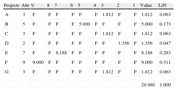
2nd stage: Add the minimum criteria attribute to the previous results to re-establish the attributes inherent value. This same procedure is applied in the case of the criteria attributes minimization and maximization, see Table 5 and Fig. 5;
Projects attribute recognition for criterion B2.
| Projects | Attr | 9 | 8 | 7 | 6 | 5 | 4 | 3 | 2 | 1 | Value | LiN |
| A | 3 | F | F | F | F | F | F | 1.812 | F | F | 1.812 | 0.063 |
| B | 5 | F | F | F | F | 5.000 | F | F | F | F | 5.000 | 0.173 |
| C | 3 | F | F | F | F | F | F | 1.812 | F | F | 1.812 | 0.063 |
| D | 2 | F | F | F | F | F | F | F | 1.356 | F | 1.356 | 0.047 |
| E | 7 | F | F | 8.188 | F | F | F | F | F | F | 8.188 | 0.283 |
| F | 9 | 9.000 | F | F | F | F | F | F | F | F | 9.000 | 0.311 |
| G | 3 | F | F | F | F | F | F | 1.812 | F | F | 1.812 | 0.063 |
| 28.980 | 1.000 | |||||||||||
Projects=R&D projects (our options).
Attr=criterion attribute value of all the projects, see Table 3.
Value=options actual value.
F=false, when the recognition condition connecting Tables 4 and 5 doesn’t find any correspondence.
LiN=corresponds to the linear normalization to attain the options relative value.
3rd stage: Establish an automated procedure to recognize the projects attribute on the column “Value” of Table 6. This stage is represented in Table 5;
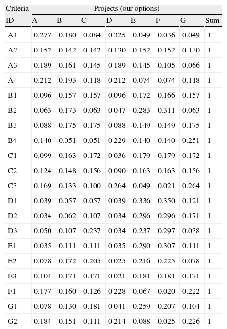
Projects value on every criterion.
| Criteria | Projects (our options) | |||||||
| ID | A | B | C | D | E | F | G | Sum |
| A1 | 0.277 | 0.180 | 0.084 | 0.325 | 0.049 | 0.036 | 0.049 | 1 |
| A2 | 0.152 | 0.142 | 0.142 | 0.130 | 0.152 | 0.152 | 0.130 | 1 |
| A3 | 0.189 | 0.161 | 0.145 | 0.189 | 0.145 | 0.105 | 0.066 | 1 |
| A4 | 0.212 | 0.193 | 0.118 | 0.212 | 0.074 | 0.074 | 0.118 | 1 |
| B1 | 0.096 | 0.157 | 0.157 | 0.096 | 0.172 | 0.166 | 0.157 | 1 |
| B2 | 0.063 | 0.173 | 0.063 | 0.047 | 0.283 | 0.311 | 0.063 | 1 |
| B3 | 0.088 | 0.175 | 0.175 | 0.088 | 0.149 | 0.149 | 0.175 | 1 |
| B4 | 0.140 | 0.051 | 0.051 | 0.229 | 0.140 | 0.140 | 0.251 | 1 |
| C1 | 0.099 | 0.163 | 0.172 | 0.036 | 0.179 | 0.179 | 0.172 | 1 |
| C2 | 0.124 | 0.148 | 0.156 | 0.090 | 0.163 | 0.163 | 0.156 | 1 |
| C3 | 0.169 | 0.133 | 0.100 | 0.264 | 0.049 | 0.021 | 0.264 | 1 |
| D1 | 0.039 | 0.057 | 0.057 | 0.039 | 0.336 | 0.350 | 0.121 | 1 |
| D2 | 0.034 | 0.062 | 0.107 | 0.034 | 0.296 | 0.296 | 0.171 | 1 |
| D3 | 0.050 | 0.107 | 0.237 | 0.034 | 0.237 | 0.297 | 0.038 | 1 |
| E1 | 0.035 | 0.111 | 0.111 | 0.035 | 0.290 | 0.307 | 0.111 | 1 |
| E2 | 0.078 | 0.172 | 0.205 | 0.025 | 0.216 | 0.225 | 0.078 | 1 |
| E3 | 0.104 | 0.171 | 0.171 | 0.021 | 0.181 | 0.181 | 0.171 | 1 |
| F1 | 0.177 | 0.160 | 0.126 | 0.228 | 0.067 | 0.020 | 0.222 | 1 |
| G1 | 0.078 | 0.130 | 0.181 | 0.041 | 0.259 | 0.207 | 0.104 | 1 |
| G2 | 0.184 | 0.151 | 0.111 | 0.214 | 0.088 | 0.025 | 0.226 | 1 |
As we can see, on the example of Table 5, for the criterion B2, the project A has an a punctuation of 3 points, which corresponds to an importance value of 1.812 in Table 4. If we check the other projects we can notice that the projects punctuation has been converted into a value expressing the decision-maker perceptions on the column “Value”;
4th stage: Establish the linear normalization of the column “Value”, of Table 5, by applying formula (2):
The linear normalization converts the different values into the same scale, the addition of all the values sums one (see Table 5).
If we perform the same procedure for all the criteria we’re going to attain the projects relative value on all the criteria, as presented in Table 6:
At this stage, we know the relative value of every project on every criterion, but we cannot decide which project is the best since the criteria may have different weights. So the next step, to determine the projects value, is the one combining the projects value on every criterion with its relative weight. But before this last step, it is important to make a remark concerning the utility functions of the measuring scales in use.
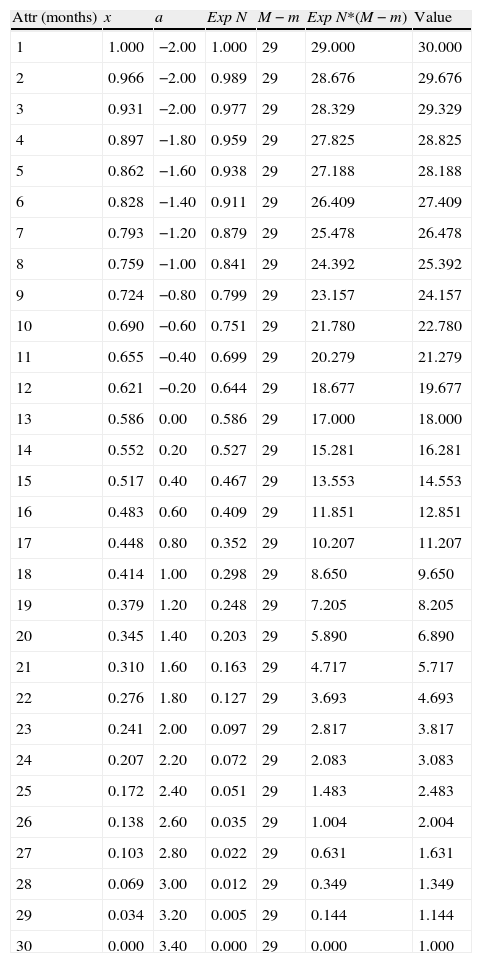
Remark: In the case of criterion B2 we had a reference scale between 1 and 9, being the best condition the highest value. However, we can have reference scales with different dimensions and conditions. For example, the criterion C3 (time needed to display a marketable technology with all the required industrial and legal specifications), is displayed in an horizon of 30 months and the best condition is the lowest value, see Table 7.
Utility function for the attributes value of criterion C3 – time needed to display a marketable technology with all the required industrial and legal specifications.
| Attr (months) | x | a | ExpN | M−m | ExpN*(M−m) | Value |
| 1 | 1.000 | −2.00 | 1.000 | 29 | 29.000 | 30.000 |
| 2 | 0.966 | −2.00 | 0.989 | 29 | 28.676 | 29.676 |
| 3 | 0.931 | −2.00 | 0.977 | 29 | 28.329 | 29.329 |
| 4 | 0.897 | −1.80 | 0.959 | 29 | 27.825 | 28.825 |
| 5 | 0.862 | −1.60 | 0.938 | 29 | 27.188 | 28.188 |
| 6 | 0.828 | −1.40 | 0.911 | 29 | 26.409 | 27.409 |
| 7 | 0.793 | −1.20 | 0.879 | 29 | 25.478 | 26.478 |
| 8 | 0.759 | −1.00 | 0.841 | 29 | 24.392 | 25.392 |
| 9 | 0.724 | −0.80 | 0.799 | 29 | 23.157 | 24.157 |
| 10 | 0.690 | −0.60 | 0.751 | 29 | 21.780 | 22.780 |
| 11 | 0.655 | −0.40 | 0.699 | 29 | 20.279 | 21.279 |
| 12 | 0.621 | −0.20 | 0.644 | 29 | 18.677 | 19.677 |
| 13 | 0.586 | 0.00 | 0.586 | 29 | 17.000 | 18.000 |
| 14 | 0.552 | 0.20 | 0.527 | 29 | 15.281 | 16.281 |
| 15 | 0.517 | 0.40 | 0.467 | 29 | 13.553 | 14.553 |
| 16 | 0.483 | 0.60 | 0.409 | 29 | 11.851 | 12.851 |
| 17 | 0.448 | 0.80 | 0.352 | 29 | 10.207 | 11.207 |
| 18 | 0.414 | 1.00 | 0.298 | 29 | 8.650 | 9.650 |
| 19 | 0.379 | 1.20 | 0.248 | 29 | 7.205 | 8.205 |
| 20 | 0.345 | 1.40 | 0.203 | 29 | 5.890 | 6.890 |
| 21 | 0.310 | 1.60 | 0.163 | 29 | 4.717 | 5.717 |
| 22 | 0.276 | 1.80 | 0.127 | 29 | 3.693 | 4.693 |
| 23 | 0.241 | 2.00 | 0.097 | 29 | 2.817 | 3.817 |
| 24 | 0.207 | 2.20 | 0.072 | 29 | 2.083 | 3.083 |
| 25 | 0.172 | 2.40 | 0.051 | 29 | 1.483 | 2.483 |
| 26 | 0.138 | 2.60 | 0.035 | 29 | 1.004 | 2.004 |
| 27 | 0.103 | 2.80 | 0.022 | 29 | 0.631 | 1.631 |
| 28 | 0.069 | 3.00 | 0.012 | 29 | 0.349 | 1.349 |
| 29 | 0.034 | 3.20 | 0.005 | 29 | 0.144 | 1.144 |
| 30 | 0.000 | 3.40 | 0.000 | 29 | 0.000 | 1.000 |
From Table 7 we can see that the utility function of the attributes of criterion C3 have been inverted and modified on the column “Value” in accordance to the decision-maker perceptions. The same minimization condition is applied for the criterion F1 (Investment and operational additional costs with the R&D project after discounting public funds (if available)) and for the criterion G2 (Expected pay-back period).
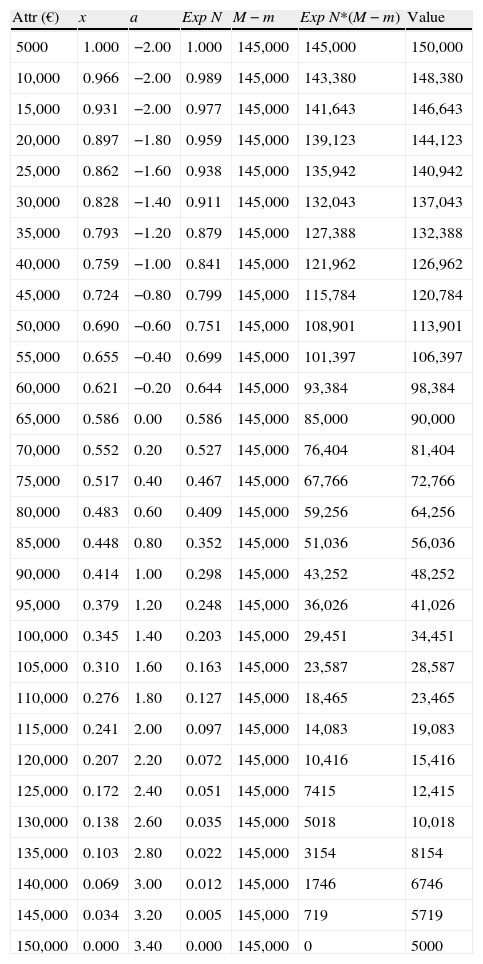
On the criterion F1 (Investment and operational additional costs with the R&D project after discounting public funds (if available)) instead of having a sequence of values representing the reference scale, we have intervals, and this is represented in Table 8.
Utility function for the attributes value of criterion F1 – investment and operational additional costs with the R&D project after discounting public funds (if available).
| Attr (€) | x | a | ExpN | M−m | ExpN*(M−m) | Value |
| 5000 | 1.000 | −2.00 | 1.000 | 145,000 | 145,000 | 150,000 |
| 10,000 | 0.966 | −2.00 | 0.989 | 145,000 | 143,380 | 148,380 |
| 15,000 | 0.931 | −2.00 | 0.977 | 145,000 | 141,643 | 146,643 |
| 20,000 | 0.897 | −1.80 | 0.959 | 145,000 | 139,123 | 144,123 |
| 25,000 | 0.862 | −1.60 | 0.938 | 145,000 | 135,942 | 140,942 |
| 30,000 | 0.828 | −1.40 | 0.911 | 145,000 | 132,043 | 137,043 |
| 35,000 | 0.793 | −1.20 | 0.879 | 145,000 | 127,388 | 132,388 |
| 40,000 | 0.759 | −1.00 | 0.841 | 145,000 | 121,962 | 126,962 |
| 45,000 | 0.724 | −0.80 | 0.799 | 145,000 | 115,784 | 120,784 |
| 50,000 | 0.690 | −0.60 | 0.751 | 145,000 | 108,901 | 113,901 |
| 55,000 | 0.655 | −0.40 | 0.699 | 145,000 | 101,397 | 106,397 |
| 60,000 | 0.621 | −0.20 | 0.644 | 145,000 | 93,384 | 98,384 |
| 65,000 | 0.586 | 0.00 | 0.586 | 145,000 | 85,000 | 90,000 |
| 70,000 | 0.552 | 0.20 | 0.527 | 145,000 | 76,404 | 81,404 |
| 75,000 | 0.517 | 0.40 | 0.467 | 145,000 | 67,766 | 72,766 |
| 80,000 | 0.483 | 0.60 | 0.409 | 145,000 | 59,256 | 64,256 |
| 85,000 | 0.448 | 0.80 | 0.352 | 145,000 | 51,036 | 56,036 |
| 90,000 | 0.414 | 1.00 | 0.298 | 145,000 | 43,252 | 48,252 |
| 95,000 | 0.379 | 1.20 | 0.248 | 145,000 | 36,026 | 41,026 |
| 100,000 | 0.345 | 1.40 | 0.203 | 145,000 | 29,451 | 34,451 |
| 105,000 | 0.310 | 1.60 | 0.163 | 145,000 | 23,587 | 28,587 |
| 110,000 | 0.276 | 1.80 | 0.127 | 145,000 | 18,465 | 23,465 |
| 115,000 | 0.241 | 2.00 | 0.097 | 145,000 | 14,083 | 19,083 |
| 120,000 | 0.207 | 2.20 | 0.072 | 145,000 | 10,416 | 15,416 |
| 125,000 | 0.172 | 2.40 | 0.051 | 145,000 | 7415 | 12,415 |
| 130,000 | 0.138 | 2.60 | 0.035 | 145,000 | 5018 | 10,018 |
| 135,000 | 0.103 | 2.80 | 0.022 | 145,000 | 3154 | 8154 |
| 140,000 | 0.069 | 3.00 | 0.012 | 145,000 | 1746 | 6746 |
| 145,000 | 0.034 | 3.20 | 0.005 | 145,000 | 719 | 5719 |
| 150,000 | 0.000 | 3.40 | 0.000 | 145,000 | 0 | 5000 |
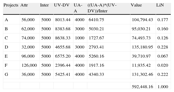
The intervals of the utility function for the criterion F1 are displayed with a width of 5000.00€. However, we can notice that the projects have investment costs within the reference interval. Since we want to consider those values, we have to follow the procedure described in Table 9.
Projects attribute recognition for criterion F1.
| Projects | Attr | Inter | UV-DV | UA-A | ((UA-A)*(UV-DV))/Inter | Value | LiN |
| A | 56,000 | 5000 | 8013.44 | 4000 | 6410.75 | 104,794.43 | 0.177 |
| B | 62,000 | 5000 | 8383.68 | 3000 | 5030.21 | 95,030.21 | 0.160 |
| C | 74,000 | 5000 | 8638.33 | 1000 | 1727.67 | 74,493.73 | 0.126 |
| D | 32,000 | 5000 | 4655.68 | 3000 | 2793.41 | 135,180.95 | 0.228 |
| E | 96,000 | 5000 | 6575.20 | 4000 | 5260.16 | 39,710.97 | 0.067 |
| F | 126,000 | 5000 | 2396.44 | 4000 | 1917.16 | 11,935.42 | 0.020 |
| G | 36,000 | 5000 | 5425.41 | 4000 | 4340.33 | 131,302.46 | 0.222 |
| 592,448.16 | 1.000 | ||||||
Projects=R&D projects (our options).
Attr=criterion attribute value of every project, see Table 3.
Inter=Interval width.
UV-DV=Best value condition of the reference interval on the column “Value” of Table 8 (Up) minus (−) the Least performing value condition of the reference interval on the column “Value” of Table 8 (Down)
UA-A=Best value condition of the reference interval on the column “Attr” of Table 8 (Up) less (−) the project attribute on the column “Attr” of Table 9 (Attribute).
((UA-A)*(UV-DV))/Inter=corresponds to the intermediate value above the best value condition of the interval.
Value=((UA-A)*(UV-DV))/Inter+Best value condition of the interval given by the column “Value” of Table 8.
LiN=corresponds to the linear normalization to attain the projects relative value.
In Table 9 we have the procedure description to determine the projects value when we have utility functions represented by intervals. In this case, we were able to determine the projects relative value for criterion F1.
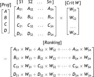
9th Attain the projects value by applying formula (3);
[Proj]=R&D projects (our options)
[Sn]=criterion attribute of the utility function
[Crit W]=criterion relative weight
The projects value is attained by multiplying their criterion attributes by the criterion weight. The projects value in our numerical example is presented in Table 10.
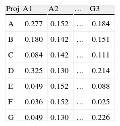
Projects proportional value.
| Proj | A1 | A2 | … | G3 |
| A | 0.277 | 0.152 | … | 0.184 |
| B | 0.180 | 0.142 | … | 0.151 |
| C | 0.084 | 0.142 | … | 0.111 |
| D | 0.325 | 0.130 | … | 0.214 |
| E | 0.049 | 0.152 | … | 0.088 |
| F | 0.036 | 0.152 | … | 0.025 |
| G | 0.049 | 0.130 | … | 0.226 |
| Crit | Weight |
| A1 | 2 |
| A2 | 2 |
| A3 | 3 |
| A4 | 3 |
| B1 | 3 |
| B2 | 2 |
| B3 | 2 |
| … | … |
| G1 | 28 |
| G2 | 10 |
| Proj | Ranking | Δ% |
| A | 12.05 | 68.39 |
| B | 14.45 | 82.01 |
| C | 14.62 | 82.97 |
| D | 11.30 | 64.09 |
| E | 17.63 | 100.00 |
| F | 14.93 | 84.72 |
| G | 15.02 | 85.20 |
| Sum | 100.00 |
From Table 10, we know that project E is the best investment alternative, with a relative value of 17.63%; project G is the second best, totalizing 15.02% of the value; the least performing ones are project A with 12.05% and project D with 11.30% of the criteria total value. On the column “Δ%” we have taken per reference the best investment project to determine how much the other projects differed from the best scoring project.
4Conclusion and further researchTo prioritize and select the best investment projects we developed an R&D projects evaluation matrix and a new procedure based on the PROV Exponential decision method, which uses multiple utility functions modeled to establish a common framework from which we can perform an effective assessment of numerous projects. The exponential normalization and the processes used to deal with the decision makers knowledge, preferences and purposes provide a useful support system to analyze tangible and intangible assets and intellectual capital, and it would be interesting to development further work to assess the possible interactions between the proposed decision approach and other methods addressing game theory and automated systems modeling.
| Grade | Criteria assessment metrics |
| A1 | Previous R&D results supporting the need and value of further research |
| 9 | Completed and validated projects supporting the need and value of further research |
| 8 | |
| 7 | Completed previous R&D results supporting the need and value of further research |
| 6 | |
| 5 | Projects in progress supporting the need and value of further research |
| 4 | |
| 3 | Generic results supporting the need and value of further research |
| 2 | |
| 1 | Absence of previous projects |
| A2 | Engaged and motivated R&D team |
| 9 | Motivated, engaged and consolidated team |
| 8 | |
| 7 | Engaged and consolidated team |
| 6 | |
| 5 | Consolidated team |
| 4 | |
| 3 | Elements not fully involved |
| 2 | |
| 1 | Dispersed team |
| A3 | Availability of a scientific research team properly answering to the R&D requisites |
| 9 | Excellent knowledge and skills to answer to the R&D requisites |
| 8 | |
| 7 | Very good knowledge and skills to answer to the R&D project requisites |
| 6 | |
| 5 | Good knowledge and skills to answer to the R&D project requisites |
| 4 | |
| 3 | Basic knowledge and skills to answer to the R&D project requisites |
| 2 | |
| 1 | Insipient knowledge and skills to answer to the R&D project requisites |
| A4 | Available infrastructures and equipments for the R&D project development at the institution |
| 9 | Fully available infrastructures and equipments |
| 8 | |
| 7 | Not fully available but easily accessible |
| 6 | |
| 5 | Non available but accessible infrastructures and equipments |
| 4 | |
| 3 | Non available at the institution and difficult to access |
| 2 | |
| 1 | Non available at the institution and very difficult to access infrastructures and equipments |
| B1 | Uniqueness of the technology (new or better performing) |
| 9 | Expected R&D completely new applications |
| 8 | |
| 7 | Expected incremental high improvement |
| 6 | |
| 5 | Expected incremental medium improvement |
| 4 | |
| 3 | Expected incremental small improvement |
| 2 | |
| 1 | Uncertain solutions and quality improvements |
| B2 | Possibility of attaining patentable results |
| 9 | Expected fully patentable technology |
| 8 | |
| 7 | Partially patentable technology |
| 6 | |
| 5 | Patentable results foreseen |
| 4 | |
| 3 | Unlikely patentable results |
| 2 | |
| 1 | Non patentable results |
| B3 | R&D final applications ability to be manufactured or used at a high industrial scale |
| 9 | Expected applications with a very high ability to be manufactured or used under the required industrial standards |
| 8 | |
| 7 | Expected applications with a high ability to be industrially manufactured or used |
| 6 | |
| 5 | Expected application with a medium ability to be industrially manufactured or used |
| 4 | |
| 3 | Expected applications with a small ability to be industrially manufactured or used |
| 2 | |
| 1 | Applications with significant industrial reproduction or use barriers |
| B4 | R&D final applications friendly-use |
| 9 | Intuitive use and operationality |
| 8 | |
| 7 | Generally trained users |
| 6 | |
| 5 | Specially trained users |
| 4 | |
| 3 | Highly skilled users |
| 2 | |
| 1 | Difficult use and operationality |
| C1 | Resulting applications clearly defined and relevant for the institution operational and expansion activities |
| 9 | Clearly established final functionalities with very high relevant use for the institution operational and expansion activities |
| 8 | |
| 7 | Well defined R&D purposes and final functionalities with high relevant use for the institution operational and expansion activities |
| 6 | |
| 5 | Well defined purposes and final functionalities with medium relevant use for the institution operational and expansion activities |
| 4 | |
| 3 | Basic definition of final functionalities with relevant use for the institution operational and expansion activities |
| 2 | |
| 1 | Unclear final functionalities |
| C2 | Perceived expressions of interest on the R&D results coming from the industry sector |
| 9 | Expression of interest by several companies and stakeholders |
| 8 | |
| 7 | Expression of interest by a significant number of companies and stakeholders |
| 6 | |
| 5 | Expression of interest by a few companies and a significant number of stakeholders |
| 4 | |
| 3 | Expression of interest by a few stakeholders |
| 2 | |
| 1 | No existent expressions of interest |
| C3 | Time needed to display a marketable technology with all the required industrial and legal specifications |
| Expected time in months (no scale required or can be created case by case) | |
| D1 | Existence of competitor research projects and research teams clearly oriented to the R&D particular technology field |
| 9 | Absence of relevant research projects and teams oriented to the R&D particular technology field |
| 8 | |
| 7 | High demanding knowledge and skills and lack of relevant research projects and teams oriented to the R&D particular technology field |
| 6 | |
| 5 | Presence of competitor research projects and teams on the field but not focused on the R&D particular characteristics |
| 4 | |
| 3 | Some projects and research teams starting to focus on the R&D particular technology field |
| 2 | |
| 1 | Present competing research projects and teams clearly oriented to the R&D particular technology field |
| D2 | Available financial sources for competing R&D teams to pursue similar results to the ones pursued by the R&D project |
| 9 | Non-available public funding for competing R&D projects and private financial sources difficult to attain |
| 8 | |
| 7 | Self-financing with possible minor public or private funding |
| 6 | |
| 5 | Self-financing with relevant public or private funding |
| 4 | |
| 3 | Accessible public or private funding without significant self-financing efforts |
| 2 | |
| 1 | Public funding 100% available for competing R&D projects |
| D3 | Available infrastructures and equipments for competing teams to pursue similar results to the ones pursued by the R&D project |
| 9 | Advanced equipments required and very restricted access to be attained by competitor research teams |
| 8 | |
| 7 | Restricted access to infrastructures and equipments for competing teams to pursue similar results to the ones pursued by the R&D project |
| 6 | |
| 5 | Partially available infrastructures and equipments for competing teams to pursue similar results to the ones pursued by the R&D project |
| 4 | |
| 3 | Advanced equipments required but easily accessible to competing R&D teams |
| 2 | |
| 1 | Non required or fully available infrastructures and equipments for competing teams to pursue similar results to the ones pursued by the R&D project |
| E1 | Available concurrent R&D results with a similar purpose as the ones pursued by the R&D project |
| 9 | Non available concurrent R&D results with similar purposes as the ones pursued by the R&D project |
| 8 | |
| 7 | Insipient available R&D results with similar purposes as the ones pursued by the R&D project |
| 6 | |
| 5 | Partially available R&D results with similar purposes as the ones pursued by the R&D project |
| 4 | |
| 3 | Announced R&D results with similar purposes as the ones pursued by the R&D project coming to market |
| 2 | |
| 1 | Current R&D results with the similar purpose as the ones pursued by the R&D project |
| E2 | Available competing patents and publications |
| 9 | Non available or very insipient specific competing patents on the particular R&D field and non concretized publications |
| 8 | |
| 7 | Insipient available patents and publication addressing particular aspects of the R&D field |
| 6 | |
| 5 | Available patents and publications not covering the full particular R&D field |
| 4 | |
| 3 | Available patents and publications covering a major part of the R&D field |
| 2 | |
| 1 | Fully available competing patents and publications addressing the R&D project purposes |
| E3 | Current applications with similar purposes already in the market |
| 9 | Non available concurrent applications with similar purposes as the ones pursued by the R&D project in the market |
| 8 | |
| 7 | Insipient available applications with similar purposes as the ones pursued by the R&D project in the market |
| 6 | |
| 5 | Partially available applications with similar purposes as the ones pursued by the R&D project in the market |
| 4 | |
| 3 | Announced applications with similar purposes as the ones pursued by the R&D project coming to market |
| 2 | |
| 1 | Current applications with the similar purpose as the ones pursued by the R&D project in the market |
| F1 | Investment and operational additional costs with the R&D project after discounting public funds (if available) |
| Expected investment and operational additional costs in € (no scale required) | |
| G1 | NPV |
| Expected NPV (no scale required or can be created case by case) | |
| G2 | Expected pay-back period |
| Expected number of months to recover the investment and operational costs (no scale required or can be created case by case) | |


